Time series analysis is the endeavor of extracting meaningful summary and statistical information from data points that are in chronological order. They are widely used in applied science and engineering which involves temporal measurements such as signal processing, pattern recognition, mathematical finance, weather forecasting, control engineering, healthcare digitization, applications of smart cities, and so on.

時間序列分析是從按時間順序排列的數據點中提取有意義的摘要和統計信息的努力。 它們被廣泛地應用在涉及時間測量的應用科學和工程中，例如信號處理，模式識別，數學財務，天氣預報，控制工程，醫療保健數字化，智能城市的應用等。

As we are continuously monitoring and collecting time series data, the opportunities for applying time series analysis and forecasting are increasing.

隨著我們不斷監視和收集時間序列數據，應用時間序列分析和預測的機會越來越多。

In this article, I will show how to develop an ARIMA model with a seasonal component for time series forecasting in Python. We will follow Box-Jenkins three-stage modeling approach to reach at the best model for forecasting.

在本文中，我將展示如何開發帶有季節性成分的ARIMA模型，以便在Python中進行時間序列預測。 我們將遵循Box-Jenkins的三階段建模方法，以獲取最佳的預測模型。

I encourage anyone to check out the Jupyter Notebook on my GitHub for the full analysis.

我鼓勵任何人在我的GitHub上查看Jupyter Notebook進行完整分析。

In time series analysis, Box-Jenkins method named after statisticians George Box and Gwilym Jenkins applying ARIMA models to find the best fit of a time series model.

在時間序列分析中，以統計學家George Box和Gwilym Jenkins命名的Box-Jenkins方法應用ARIMA模型來找到時間序列模型的最佳擬合。

The model indicates 3 steps: model identification, parameter estimation and model validation.

該模型指示3個步驟：模型識別，參數估計和模型驗證。

時間序列 (Time Series)

As data, we will use the monthly milk production dataset. It includes monthly production records in terms of pounds per cow between 1962–1975.

作為數據，我們將使用每月牛奶產量數據集。 它包括1962年至1975年之間的月度生產記錄，以每頭母牛的磅數表示。

df = pd.read_csv('./monthly_milk_production.csv', sep=',',                            parse_dates=['Date'], index_col='Date')

時間序列數據檢查 (Time Series Data Inspection)

As we can observe from the plot above, we have an increasing trend and very strong seasonality in our data.

從上圖可以看出，我們的數據呈上升趨勢，并且季節性非常強。

We will use the statsmodels library from Python to perform a time series decomposition. The decomposition of time series is a statistical method to deconstruct time series into its trend, seasonal and residual components.

我們將使用Python中的statsmodels庫執行時間序列分解。 時間序列的分解是一種將時間序列分解為趨勢，季節和殘差成分的統計方法。

import statsmodels.api as sm
from statsmodels.tsa.seasonal import seasonal_decomposedecomposition = seasonal_decompose(df['Production'], freq=12)
decomposition.plot()
plt.show()

The decomposition plot indicates that the monthly milk production has an increasing trend and seasonal pattern.

分解圖表明，每月的牛奶產量具有增加的趨勢和季節性模式。

If we want to observe the seasonal component more precisely, we can plot the data based on the month.

如果我們想更精確地觀察季節成分，則可以根據月份繪制數據。

1.型號識別 (1. Model Identification)

In this step, we need to detect whether time series is stationary, and if not, we need to understand what kind of transformation is required to make it stationary.

在此步驟中，我們需要檢測時間序列是否穩定，如果不是，則需要了解需要哪種變換才能使其穩定。

A time series is stationary when its statistical properties such as mean, variance, and autocorrelation are constant over time. In other words, time series is stationary when it is not dependent on time and not have a trend or seasonal effects. Most statistical forecasting methods are based on the assumption that time series is (approximately) stationary.

當時間序列的統計屬性(例如均值，方差和自相關)隨時間恒定時，它是固定的。 換句話說，時間序列在不依賴時間且沒有趨勢或季節影響的情況下是固定的。 大多數統計預測方法都是基于時間序列(近似)平穩的假設。

Imagine, we have a time series that is consistently increasing over time, the sample mean and variance will grow with the size of the sample, and they will always underestimate the mean and variance in future periods. This is why, we need to start with a stationary time series, which is removed from its time dependent trend and seasonal components.

想象一下，我們有一個隨時間連續增長的時間序列，樣本均值和方差將隨樣本的大小而增長，并且它們始終會低估未來期間的均值和方差。 因此，我們需要從固定的時間序列開始，將其從與時間相關的趨勢和季節成分中刪除。

We can check stationarity by using different approaches:

我們可以使用不同的方法來檢查平穩性：

• We can understand from the plots, such as decomposition plot we have seen previously where we have already observed there is trend and seasonality.
  我們可以從圖中了解到，例如我們之前已經看到的分解圖和已經觀察到的趨勢和季節性。

• We can plot autocorrelation function and partial autocorrelation function plots, which provide information about the dependency of time series values to their previous values. If the time series is stationary, the ACF/PACF plots will show a quick cut off after a small number of lags.

  我們可以繪制自 相關函數圖和部分自相關函數圖，它們提供有關時間序列值與其先前值的相關性的信息。 如果時間序列是固定的，則ACF / PACF圖將顯示少量延遲后的快速中斷。

from statsmodels.graphics.tsaplots import plot_acf, plot_pacfplot_acf(df, lags=50, ax=ax1)
plot_pacf(df, lags=50, ax=ax2)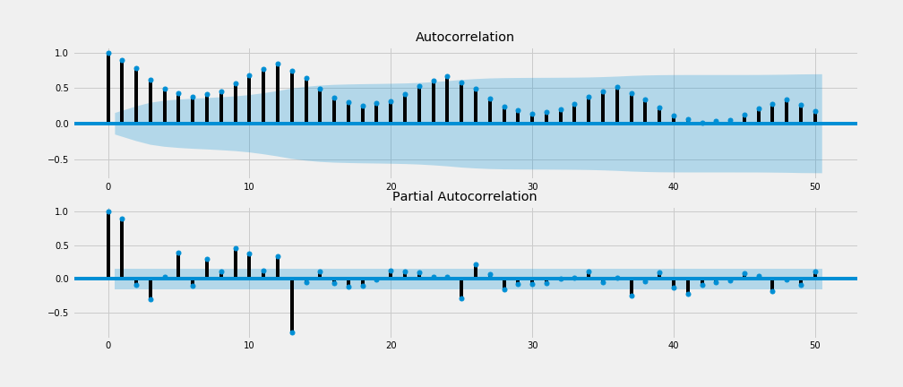

Here we see that both ACF and PACF plots do not show a quick cut off into the 95% confidence interval area (in blue) meaning time series is not stationary.

在這里，我們看到ACF和PACF圖都沒有顯示出快速切入95％置信區間區域(藍色)的意思，這意味著時間序列不是固定的。

• We can apply statistical tests and Augmented Dickey-Fuller test is the widely used one. The null hypothesis of the test is time series has a unit root, meaning that it is non-stationary. We interpret the test result using the p-value of the test. If the p-value is lower than the threshold value (5% or 1%), we reject the null hypothesis and time series is stationary. If the p-value is higher than the threshold, we fail to reject the null hypothesis and time series is non-stationary.
  我們可以應用統計檢驗，而增強Dickey-Fuller檢驗是廣泛使用的檢驗。 該檢驗的零假設是時間序列具有單位根，這意味著它是非平穩的。 我們使用測試的p值解釋測試結果。 如果p值低于閾值(5％或1％)，我們將拒絕原假設，并且時間序列是固定的。 如果p值高于閾值，則我們無法拒絕原假設，并且時間序列是非平穩的。

from statsmodels.tsa.stattools import adfullerdftest = adfuller(df['Production'])dfoutput = pd.Series(dftest[0:4], index=['Test Statistic','p-value','#Lags Used','Number of Observations Used'])
for key, value in dftest[4].items():
    dfoutput['Critical Value (%s)'%key] = value
print(dfoutput)

Results of Dickey-Fuller Test:Test Statistic -1.303812p-value 0.627427#Lags Used 13.000000Number of Observations Used 154.000000Critical Value (1%) -3.473543Critical Value (5%) -2.880498Critical Value (10%) -2.576878

Dickey-Fuller測試的結果：測試統計-1.303812p值0.627427＃使用的延遲13.000000使用的觀察數154.000000臨界值(1％)-3.473543臨界值(5％)-2.880498臨界值(10％)-2.576878

P-value is greater than the threshold value, we fail to reject the null hypothesis and time series is non-stationary, it has time dependent component.

P值大于閾值，我們無法拒絕原假設并且時間序列是非平穩的，它具有時間依賴性。

All these approaches suggest we have non-stationary data. Now, we need to find a way to make it stationary.

所有這些方法表明我們有不穩定的數據。 現在，我們需要找到一種使其固定的方法。

There are two major reasons behind non-stationary time series; trend and seasonality. We can apply differencing to make time series stationary by subtracting the previous observations from the current observations. Doing so we will eliminate trend and seasonality, and stabilize the mean of time series. Due to both trend and seasonal components, we apply one non-seasonal diff() and one seasonal differencing diff(12).

非平穩時間序列背后的主要原因有兩個： 趨勢和季節性。 通過從當前觀測值中減去先前的觀測值，我們可以應用差分來使時間序列平穩。 這樣做可以消除趨勢和季節性，并穩定時間序列的平均值。 由于趨勢和季節因素，我們應用一個非季節性diff()和一個季節性差異diff(12) 。

df_diff = df.diff().diff(12).dropna()

Results of Dickey-Fuller Test:Test Statistic -5.038002p-value 0.000019#Lags Used 11.000000Number of Observations Used 143.000000Critical Value (1%) -3.476927Critical Value (5%) -2.881973Critical Value (10%) -2.577665

Dickey-Fuller測試的結果：測試統計-5.038002p值0.000019＃使用的滯后11.000000使用的觀察數143.000000臨界值(1％)-3.476927臨界值(5％)-2.881973臨界值(10％)-2.577665

Applying the previously listed stationarity checks, we notice the plot of differenced time series does not reveal any specific trend or seasonal behavior, ACF/PACF plots have a quick cut-off, and ADF test result returns p-value almost 0.00. which is lower than the threshold. All these checks suggest that differenced data is stationary.

應用先前列出的平穩性檢查，我們注意到不同時間序列的圖沒有揭示任何特定的趨勢或季節性行為，ACF / PACF圖具有快速截止值，并且ADF測試結果返回的p值幾乎為0.00。 低于閾值。 所有這些檢查表明差異數據是固定的。

We will apply Seasonal Autoregressive Integrated Moving Average (SARIMA or Seasonal-ARIMA) which is an extension of ARIMA that supports time series data with a seasonal component. ARIMA stands for Autoregressive Integrated Moving Average which is one of the most common techniques of time series forecasting.

我們將應用季節性自回歸綜合移動平均線(SARIMA或Seasonal-ARIMA)，這是ARIMA的擴展，它支持帶有季節性成分的時間序列數據。 ARIMA代表自回歸綜合移動平均值，它是時間序列預測中最常用的技術之一。

ARIMA models are denoted with the order of ARIMA(p,d,q) and SARIMA models are denoted with the order of SARIMA(p, d, q)(P, D, Q)m.

ARIMA模型以ARIMA(p，d，q)的順序表示，而SARIMA模型以SARIMA(p，d，q)(P，D，Q)m的順序表示。

AR(p) is a regression model that utilizes the dependent relationship between an observation and some number of lagged observations.

AR(p)是一種回歸模型，利用了觀察值與一些滯后觀察值之間的依賴關系。

I(d) is the differencing order to make time series stationary.

I(d)是使時間序列平穩的微分階數。

MA(q) is a model that uses the dependency between an observation and a residual error from a moving average model applied to lagged observations.

MA(q)是一個模型，它使用觀察值與應用于滯后觀察值的移動平均模型的殘差之間的依賴關系。

(P, D, Q)m are the additional set of parameters that specifically describe the seasonal components of the model. P, D, and Q represent the seasonal regression, differencing, and moving average coefficients, and m represents the number of data points in each seasonal cycle.

(P，D，Q)m是另外一組參數，它們專門描述了模型的季節性成分。 P，D和Q表示季節回歸系數，微分系數和移動平均系數，m表示每個季節周期中數據點的數量。

2.模型參數估計 (2. Model Parameter Estimation)

We will use Python’s pmdarima library, to automatically extract the best parameters for our Seasonal ARIMA model. Inside auto_arima function, we will specify d=1and D=1 as we differentiate once for the trend and once for seasonality, m=12 because we have monthly data, and trend='C'to include constant and seasonal=Trueto fit a seasonal-ARIMA. Besides, we specify trace=Trueto print status on the fits. This helps us to determine the best parameters by comparing the AIC scores.

我們將使用Python的pmdarima庫為我們的季節性ARIMA模型自動提取最佳參數。 在auto_arima函數中，我們將指定d=1和D=1因為我們分別對趨勢和季節性進行了區分，因為我們有月度數據，所以對m=12進行了區分，并且trend='C'包含了常數， seasonal=True適合一個季節性的ARIMA。 此外，我們指定trace=True來顯示適合的打印狀態。 這可以幫助我們通過比較AIC分數來確定最佳參數。

import pmdarima as pmmodel = pm.auto_arima(df['Production'], d=1, D=1,
                      m=12, trend='c', seasonal=True, 
                      start_p=0, start_q=0, max_order=6, test='adf',
                      stepwise=True, trace=True)

AIC (Akaike Information Criterion) is an estimator of out of sample prediction error and the relative quality of our model. The desired result is to find the lowest possible AIC score.

AIC (赤池信息準則)是對樣本外預測誤差和模型相對質量的估計。 理想的結果是找到最低的AIC分數。

The result of auto_arima function with various (p, d, q)(P, D, Q)m parameters indicates that the lowest AIC score is obtained when the parameters equal to (1, 1, 0)(0, 1, 1, 12).

參數為(p，d，q)(P，D，Q)m的auto_arima函數的結果表明，當參數等于(1，1，0)(0，1，1， 12)。

We split the dataset into a train and test set. Here I’ve used 85% as train split size. We create a SARIMA model, on the train set with the suggested parameters. We use SARIMAX function from statsmodel library (X describes the exogenous parameter, but here we don’t add any). After fitting the model, we can also print the summary statistics.

我們將數據集分為訓練和測試集。 在這里，我使用了85％作為火車分割大小。 我們在火車上使用建議的參數創建SARIMA模型。 我們使用statsmodel庫中的SARIMAX函數(X描述了外部參數，但此處未添加任何參數)。 擬合模型后，我們還可以打印摘要統計信息。

from statsmodels.tsa.statespace.sarimax import SARIMAXmodel = SARIMAX(train['Production'],
                order=(1,1,0),seasonal_order=(0,1,1,12))
results = model.fit()
results.summary()

3.模型驗證 (3. Model Validation)

Primary concern of the model is to ensure that the residuals are normally distributed with zero mean and uncorrelated.

該模型的主要關注點是確保殘差正態分布且均值為零且不相關。

To check for residuals statistics, we can print model diagnostics:

要檢查殘差統計信息，我們可以打印模型診斷：

results.plot_diagnostics()
plt.show()

• The top-left plot shows the residuals over time and it appears to be a white noise with no seasonal component.
  左上方的圖顯示了隨時間變化的殘差，它似乎是白噪聲，沒有季節性成分。
• The top-right plot shows that kde line (in red) closely follows the N(0,1) line, which is the standard notation of normal distribution with zero mean and standard deviation of 1, suggesting the residuals are normally distributed.
  右上圖顯示kde線(紅色)緊跟N(0,1)線，這是正態分布的標準表示法，均值為零，標準差為1，表明殘差呈正態分布。
• The bottom-left normal gg-plot shows ordered distribution of residuals (in blue) closely follow the linear trend of the samples taken from a standard normal distribution, suggesting residuals are normally distributed.
  左下方正態gg曲線顯示殘差的有序分布(藍色)緊密遵循從標準正態分布獲取的樣本的線性趨勢，表明殘差呈正態分布。
• The bottom-right is a correlogram plot indicating residuals have a low correlation with lagged versions.
  右下角是相關圖，表明殘差與滯后形式的相關性較低。

All these results suggest residuals are normally distributed with low correlation.

所有這些結果表明殘差正態分布且相關性較低。

To measure the accuracy of forecasts, we compare the prediction values on the test set with its real values.

為了衡量預測的準確性，我們將測試集上的預測值與其實際值進行比較。

forecast_object = results.get_forecast(steps=len(test))
mean = forecast_object.predicted_mean
conf_int = forecast_object.conf_int()
dates = mean.index

From the plot, we see that model prediction nearly matches with the real values of the test set.

從圖中可以看出，模型預測幾乎與測試集的實際值匹配。

from sklearn.metrics import r2_scorer2_score(test['Production'], predictions)>>> 0.9240433686806808

The R squared of the model is 0.92, indicating that the coefficient of determination of the model is 92%.

該模型的R平方為0.92，表明該模型的確定系數為92％。

mean_absolute_percentage_error = np.mean(np.abs(predictions - test['Production'])/np.abs(test['Production']))*100>>> 1.649905

Mean absolute percentage error (MAPE) is one of the most used accuracy metrics, expressing the accuracy as a percentage of the error. MAPE score of the model equals to 1.64, indicating the forecast is off by 1.64% and 98.36% accurate.

平均絕對百分比誤差 (MAPE)是最常用的精度指標之一，將精度表示為誤差的百分比。 該模型的MAPE得分等于1.64，表明預測的準確度為1.64％和98.36％。

Since both the diagnostic test and the accuracy metrics intimates that our model is nearly perfect, we can continue to produce future forecasts.

由于診斷測試和準確性指標都表明我們的模型幾乎是完美的，因此我們可以繼續產生未來的預測。

Here is the forecast for the next 60 months.

這是對未來60個月的預測。

results.get_forecast(steps=60)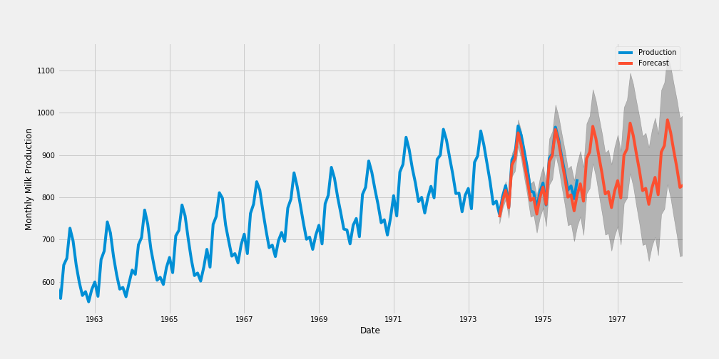

I hope you enjoyed following this tutorial and building time series forecasts in Python.

我希望您喜歡本教程并使用Python建立時間序列預測。

Let me know if you have any questions or suggestions.?

如果您有任何問題或建議，請告訴我。?