Note from Towards Data Science’s editors: While we allow independent authors to publish articles in accordance with our rules and guidelines, we do not endorse each author’s contribution. You should not rely on an author’s works without seeking professional advice. See our Reader Terms for details.

Towards Data Science編輯的注意事項： 雖然我們允許獨立作者按照我們的 規則和指南 發表文章 ，但我們不認可每位作者的貢獻。 您不應在未征求專業意見的情況下依賴作者的作品。 有關 詳細信息， 請參見我們的 閱讀器條款 。

Maybe you’re an investor trying to decide whether a stock is worth investing in. Maybe you’ve only recently heard of Bayesian inference and want to get a sense of how it can be applied in the real world. Maybe you’re a seasoned analyst who stumbled upon this article and found the title interesting. Regardless of where you come from, I thank you for giving this piece a read. I’m going to talk about the normal-normal model, one of the foundational models in Bayesian statistics, and how it can be used to estimate the growth rate of a company’s revenue. That estimate can then be used to decide whether or not the company is a worthwhile investment.

也許您是試圖確定股票是否值得投資的投資者。也許您只是最近才聽說過貝葉斯推理，并想了解如何將其應用到現實世界中。 也許您是一位經驗豐富的分析師，偶然發現了這篇文章，并發現標題很有趣。 無論您來自何處，我都感謝您閱讀本文。 我將討論貝葉斯統計中的基本模型之一，正常-正常模型，以及如何將其用于估計公司收入的增長率。 然后，可以使用該估算值來確定公司是否值得投資。

The first objective of this piece is to demonstrate how the normal-normal model can be used to incorporate a subjective overlay into data analysis. The second is to provide some intuition behind the normal-normal model and Bayesian inference in general without getting too bogged down in the mechanics. I’ll say it here and again at the end of the article, but this piece does not constitute investment advice. It is meant to be educational.

本文的第一個目的是演示如何使用正常-正常模型將主觀疊加納入數據分析。 第二個目的是在法線-法線模型和貝葉斯推理之后提供一些直覺，而又不會過于迷惑力學。 我將在本文的結尾處一再說，但這并不構成投資建議。 這是為了教育。

With that disclaimer out of the way, let’s get to it!

有了這個免責聲明，讓我們開始吧！

手頭的任務 (The Task at Hand)

Financial modeling generally refers to projecting fundamental values for a company in order to arrive at a fair price estimate for the company’s stock. Some of the most common metrics used to arrive at valuations are revenue, earnings, and cash flow. The company we’re going to look at is MongoDB, a software services company. It began trading publicly back in 2017, and its revenue growth has been tremendous.

財務建模通常是指預測公司的基本價值，以便得出公司股票的合理價格估計。 用于得出估值的一些最常見的指標是收入，收益和現金流量。 我們要看的公司是軟件服務公司MongoDB。 它于2017年開始公開交易，其收入增長巨大。

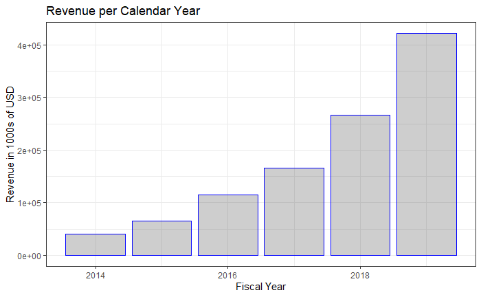
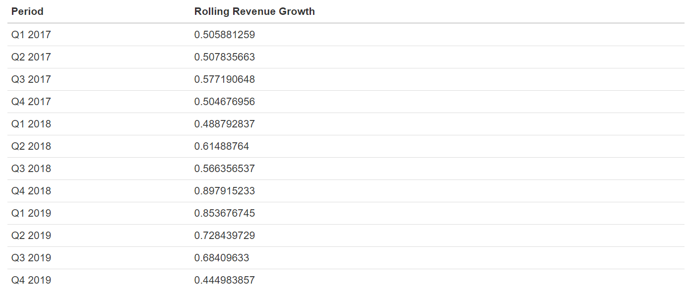
Given how young the company is and how it’s in a growth-oriented phase of its existence, it’s reasonable to focus on revenue in order to value the company. Data in the company’s 10-K filings, the annual financial reports, shows revenue numbers on a quarterly basis starting in fiscal 2016. Annual numbers are present from the year 2014. To give us more data than the six annual numbers (which translate into five growth numbers), I’ve computed rolling one-year revenue growth on a quarterly basis. That data is shown below.

考慮到公司的年輕程度以及它處于生存發展階段的方式，合理地關注收入以對公司進行估值是合理的。 該公司10-K檔案(年度財務報告)中的數據顯示了從2016財年開始的季度收入數字。從2014年開始提供年度數字。為我們提供的數據要比六個年度數字(這意味著五個增長數字)，我已經計算出了一個季度滾動的一年收入增長。 該數據如下所示。

Closer to the end of this piece, I’ll compare the results of our analysis using year-end data versus quarterly data. (Although I haven’t run a formal analysis, I assume there’s a degree of serial correlation in the quarterly data. This won’t matter in terms of explaining the concepts of the normal-normal model, but it is certainly something to be mindful of in practice.)

在本文的最后，我將比較使用年末數據和季度數據進行分析的結果。 (盡管我沒有進行正式的分析，但我假設季度數據中存在一定程度的序列相關性。這在解釋法線-法線模型的概念方面并不重要，但一定要注意在實踐中。)

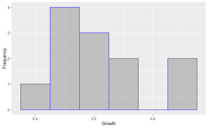
A common way to project revenue for a company is to use the average historical revenue growth rate over a certain amount of time. For companies with many years of data, this isn’t necessarily a bad practice, especially if the growth rates follow a normal distribution. Given how little sample data we have and the histogram of the data which I’ll plot below, we may feel that using the sample mean in this case is unwise.

預測公司收入的一種常用方法是使用一定時間內的平均歷史收入增長率。 對于擁有多年數據的公司而言，這不一定是壞習慣，尤其是當增長率遵循正態分布時。 考慮到我們只有很少的樣本數據以及我將在下面繪制的數據直方圖，我們可能會覺得在這種情況下使用樣本均值是不明智的。

Bayesian inference is particularly useful in situations where our sample size is small and we hold a subjective belief that our sample data does not appropriately represent what a larger sample would look like.

在樣本量較小并且我們主觀認為樣本數據不能適當代表較大樣本的情況下，貝葉斯推斷特別有用。

To conduct Bayesian inference, we’ll need a prior distribution and a sampling model. Before defining those distributions in our context, I’ll go over some of the basics of Bayesian inference and how the prior distribution and sampling model come into play. Feel free to skip this section if you’re familiar with Bayes’ theorem and how it applies to distributions.

要進行貝葉斯推斷，我們需要先驗分布和采樣模型。 在我們的上下文中定義這些分布之前，我將介紹貝葉斯推斷的一些基礎知識以及先驗分布和采樣模型如何發揮作用。 如果您熟悉貝葉斯定理及其在分布中的應用，請隨時跳過本節。

貝葉斯定理和分布 (Bayes’ Theorem and Distributions)

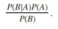
In its simplest form, Bayes’ theorem is defined as

以最簡單的形式，貝葉斯定理定義為

which is equivalent to

相當于

This is all well and good if we have neatly defined probabilities to use, but distributions complicate the process a little.

如果我們有明確定義的使用概率，那么這一切都很好，但是分布會使過程復雜化了一點。

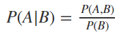
First, let’s substitute A with θ and B with Y. In this case, Y refers to the points in our sample data, and θ refers to the true average growth rate in revenue for MongoDB. Re-writing the second form of the formula with our substitutions, we have

首先，讓我們用θ替換A并用Y替換B。 在這種情況下， Y表示示例數據中的點， θ表示MongoDB的收入的真實平均增長率。 用我們的替換來重寫公式的第二種形式，我們有

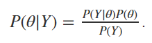
In words, the distribution we’re trying to model is the distribution of average revenue growth rate GIVEN our sample growth rates. We will use our sample data and a little bit of judgement to define this distribution P(Y|θ). We will also need a prior distribution P(θ) for our average growth rate and the marginal distribution of our data P(Y). The onus is on us to define our sampling distribution as well as define a prior distribution for θ. Once we have a sampling distribution P(Y|θ), the correct way to obtain P(Y) would be to solve for the integral below:

換句話說，我們要建模的分布是根據我們的樣本增長率得出的平均收入增長率的分布。 我們將使用樣本數據和一些判斷來定義此分布P ( Y | θ )。 對于平均增長率和數據的邊際分布P ( Y )，我們還將需要先驗分布P ( θ )。 我們有責任定義采樣分布以及θ的先驗分布。 一旦有了采樣分布P ( Y | θ )，獲得P ( Y )的正確方法就是求解以下積分：

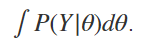
In practice, this may be difficult to do, but we can use a shortcut. Since Y is only conditional on θ in this instance, P(Y) is an unconditional probability distribution and encompasses all possibilities of Y. This means that the area under the distribution will be equal to 1 (the sum of all probabilities for an event equals 1), and the integral will be equal to 1 multiplied by a normalizing constant. Rather than solve for this normalizing constant, we can instead say

實際上，這可能很難做到，但是我們可以使用快捷方式。 由于在這種情況下Y僅以θ為條件，因此P ( Y )是無條件的概率分布，并且包含Y的所有可能性。 這意味著分布下的面積將等于1(一個事件的所有概率之和等于1)，并且積分將等于1乘以歸一化常數。 除了解決這個標準化常數外，我們可以說

P(θ|Y)∝P(Y|θ)P(θ)

P ( θ | Y )∝ P ( Y | θ ) P ( θ )

where ∝ stands for “is proportional to.” In other words, we don’t need to worry about P(Y). With one task eliminated, we only have to define our sampling and prior distributions.

∝代表“正比于”。 換句話說，我們不必擔心P ( Y )。 消除一項任務后，我們只需定義采樣和先驗分布即可。

(Note: technically, Y is conditional on sample variance. In this case, we are going to assume that the variance is known and constant. Because our variance is assumed to be known and a constant, we can omit it from the notation.)

(注意：從技術上講， Y以樣本方差為條件。在這種情況下，我們將假設方差是已知的并且是常數。因為我們的方差被假定為已知并且是常數，所以可以從符號中忽略它。)

定義我們的抽樣模型和先驗分布 (Defining Our Sampling Model and Prior Distribution)

We’re going to use a normal model for our sampling distribution. Having looked at the histogram for our data, one may think that there are distributions available to us that better represent the data. I like the normal distribution in this case because it is continuous and has support along all real numbers (revenue growth could theoretically be negative or positive).

我們將使用正常模型進行抽樣分配。 在查看了我們數據的直方圖之后，我們可能會認為有一些可用的分布更好地表示了數據。 在這種情況下，我喜歡正態分布，因為它是連續的并且在所有實數上都有支持(理論上收入增長可以是負數或正數)。

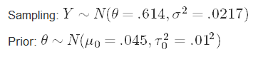
To define this sampling model, we compute the mean and variance for this data set and use these as the parameters for our sampling model. The form this will take is

為了定義該采樣模型，我們計算該數據集的均值和方差，并將其用作我們的采樣模型的參數。 采取的形式是

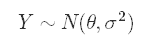
where the first term represents the unknown true average growth rate for MongoDB’s revenue and the second term represents the variance of the growth rates; we will treat this variance as known. We could just as easily assume that we know our mean but not our variance or that we know neither; all three classes of situations are well-documented and have substantial literature regarding how to work them. The normal-normal model applies to the situation with known variance and unknown mean, hence why we are making our current assumptions.

其中第一項代表MongoDB收入的未知真實平均增長率，第二項代表增長率的方差； 我們將這種差異視為已知。 我們可以很容易地假設我們知道我們的平均值，但是我們不知道方差，或者我們都不知道。 這三類情況都有充分的文獻記錄，并有大量有關如何工作的文獻。 正常-正常模型適用于方差已知且均值未知的情況，因此我們為什么要進行當前的假設。

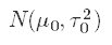
Next, we need to define a prior distribution for θ. For the same reasons that we’re using a normal distribution for the sampling model (continuous, support along positive and negative values), we’re going to use a normal distribution as our prior. We need to define a mean and a variance for the variable θ. We’ll define this distribution as

接下來，我們需要定義θ的先驗分布。 出于同樣的原因，我們在抽樣模型中使用正態分布(連續的，沿正值和負值的支持)，因此我們將使用正態分布作為先驗。 我們需要為變量θ定義均值和方差。 我們將這種分布定義為

where the first term is the prior mean and the second term is the prior variance. There is significant literature dedicated to selecting priors; the main focus of this piece is how to apply the normal-normal model, so I didn’t put extensive effort in defining my prior distribution.

其中第一項是先驗均值，第二項是先驗方差。 有大量文獻致力于選擇先驗。 本文的主要重點是如何應用正態-正態模型，因此我沒有花太多精力來定義我的先前分布。

To select a value for the prior mean, I looked at the average revenue growth rate of sales of the S&P 500 index over the last 19 years (multpl.com) and then multiplied it by the β of MongoDB. In the world of equities, β refers to the covariance of an individual stock’s returns with the return of broader basket of stocks (often called an index) divided by the variance of the index returns. MongoDB has a β of about 1.26 according to Seeking Alpha, a research site with news, data, and analyses of many stocks. Whenever we see a β > 1, we can assume that the stock we are looking at is more volatile than the index it is being compared to; for this reason, I multiply the revenue growth of the index by β. Other approaches could involve looking at slightly older companies in the software service industries or similar age companies across industries. No method is perfect, and all are viable.

為了為先前的均值選擇一個值，我查看了標普500指數過去19年的平均銷售收入增長率(multpl.com) ，然后將其乘以MongoDB的β。 在股票世界中，β指的是單個股票收益與更廣泛的一籃子股票(通常稱為指數)的收益除以指數收益的方差的協方差。 根據提供新聞，數據和許多股票分析的研究網站Seeking Alpha的數據，MongoDB的β約為1.26。 每當我們看到β> 1時，我們就可以假設我們所看的股票的波動性大于它所比較的??指數； 因此，我將指數的收入增長乘以β。 其他方法可能涉及查看軟件服務行業中稍老的公司或跨行業的類似年齡的公司。 沒有一種方法是完美的，并且所有方法都是可行的。

The next parameter we have to assign is the prior variance. Just to be clear, this is not what we presume is the variance in growth rates, but the presumed variance of the AVERAGE growth rate; this prior variance is meant to reflect our certainty in the accuracy of the prior mean. If we had full confidence that this was the correct mean to use, we could set our variance effectively equal to 0 (for computation purposes, we can’t actually use 0, but we can use a very small number such as .00001). On the other hand, if we have very little confidence in our estimate, we can use a large variance to indicate this level of certainty. In this case, where our prior mean is about 4.5%, I don’t have much of an opinion of how confident I am with this estimate. To define my distribution, I’ll use a standard deviation of 10%. With this, I’m effectively stating that I’m 95% confident that the true value for theta lies between -15.5% and 24.5% (4.5+/-2 standard deviations). This estimate may seem highly conservative given how MongoDB’s average growth rate has been about 61%, but this is exactly why Bayesian inference is powerful. MongoDB has spent the majority of its time trading in a bull market that was particularly favorable for software names. The prior distribution reflects data from multiple market cycles and consequently multiple phases of growth and contraction. Between the possibility of economic contraction, the chance MongoDB doesn’t execute its strategy effectively, and revenue growth slowing simply due to scale, I’m holding the subjective belief that MongoDB’s true average growth rate is less than what the sample data suggests. The prior distribution I’ve selected represents that belief. Now, we can study the output of our analysis.

我們必須分配的下一個參數是先驗方差。 需要明確的是，這不是我們所假定的增長率的方差，而是假定的平均增長率的方差。 此先驗方差旨在反映我們對先驗均值準確性的確定性。 如果我們完全有信心使用這是正確的平均值，則可以將方差有效地設置為0(出于計算目的，我們實際上不能使用0，但是可以使用非常小的數字，例如.00001)。 另一方面，如果我們對估計的信心很小，則可以使用較大的方差來表示此確定性級別。 在這種情況下，我們之前的均值約為4.5％，我對這個估計有多自信沒有多少看法。 為了定義我的分布，我將使用10％的標準偏差。 借此，我有效地表明，我有95％的信心認為theta的真實值在-15.5％和24.5％之間(4.5 +/- 2標準偏差)。 考慮到MongoDB的平均增長率如何達到61％左右，這個估計值似乎非常保守，但這正是貝葉斯推斷強大的原因。 MongoDB大部分時間都在牛市中交易，這對軟件名稱特別有利。 先前的分布反映了來自多個市場周期的數據，因此反映了增長和收縮的多個階段。 在經濟收縮的可能性，MongoDB無法有效執行其戰略的機會以及僅僅是由于規模而導致的收入增長放緩之間，我主觀地認為MongoDB的真實平均增長率低于樣本數據所表明的水平。 我選擇的先前分配代表了這一信念。 現在，我們可以研究分析的結果。

To recap, here are the forms for our two models:

回顧一下，這是我們兩個模型的表格：

Great, let’s move on to our analysis!

太好了，讓我們繼續進行分析！

后驗分析和直覺 (Posterior Analysis and Intuition)

I’ll focus more on the intuition offered by these forms rather than walk through a derivation by hand. Anyone truly interested in using the normal-normal model should study the derivation of the above parameters. Wikipedia has some good documentation, and most introductory textbooks to Bayesian statistics cover the derivations in detail.

我將更多地關注這些形式提供的直覺，而不是手工進行推導。 任何對使用法線-法線模型感興趣的人都應該研究上述參數的推導。 Wikipedia有一些很好的文檔，并且有關貝葉斯統計的大多數入門教科書都詳細介紹了派生方法。

When we have a normal distribution for our sampling model as well as a normal for our prior distribution on the sample mean, the resulting posterior distribution is a product of two normal models. The power of the normal-normal model is that the product of these distributions is also a normal distribution, albeit with updated parameters. In Bayesian jargon, a normal prior distribution is a conjugate prior distribution, meaning that it and its resulting posterior distribution have the same form. The fact that our posterior distribution is a normal distribution may not seem like that big of a deal, but depending on the data we’re trying to model and the parameters we’re trying to estimate, there are many instances where our posterior does not take such a familiar form. Because this posterior distribution is well-defined, we can sample from it directly and consequently compute summary statistics on it easily.

當我們的采樣模型具有正態分布，并且樣本均值具有先驗分布的正態分布時，所得后驗分布是兩個正態模型的乘積。 正態-正態模型的功效在于，盡管具有更新的參數，但這些分布的乘積也是正態分布。 在貝葉斯行話中，正態先驗分布是共軛先驗分布，這意味著它和它的后驗分布具有相同的形式。 后驗分布是正態分布這一事實似乎沒什么大不了的，但是根據我們要建模的數據和我們要估算的參數，在很多情況下我們的后驗分布不是采取這樣熟悉的形式 由于此后驗分布是定義明確的，因此我們可以直接從中進行采樣，從而輕松地計算出其后的摘要統計量。

The notations and re-parametrizations below are from Chapter 5 in Peter Hoff’s textbook, “A First Course in Bayesian Statistics,” the book I used in my first undergraduate Bayesian statistics course and the book I’ve been studying in recent times.

下面的表示法和重新參數化來自彼得·霍夫(Peter Hoff)教科書“貝葉斯統計學的第一門課程”的第5章，這是我在我的第一門貝葉斯統計學課程中使用的書，也是我最近所研究的書。

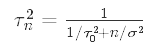
Our posterior distribution takes the form

我們的后驗分布形式為

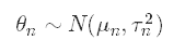
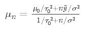
where the first term refers to the posterior mean and second term refers to the posterior variance. The formulas to calculate these updated parameters are

其中第一項指的是后均值，第二項指的是后方方差。 計算這些更新參數的公式是

and

和

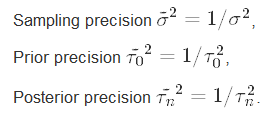
These formulas may look somewhat intimidating, but hopefully you see some similarities between them. A common practice and a particularly helpful one for gaining intuition about these formulas is to look at the formulas in terms of precision rather than variance. Precision is the inverse of variance.

這些公式可能看起來有些嚇人，但希望您能看到它們之間的相似之處。 獲得這些公式的直覺的一種常見實踐和一種特別有用的方法是，從精度而不是方差的角度來看這些公式。 精度是方差的倒數。

In this case, we have three relevant precisions to observe:

在這種情況下，我們需要觀察三個相關的精度：

If we invert the posterior variance formula to calculate posterior precision, we see that the posterior precision in terms of standard deviations is

如果我們反轉后驗方差公式以計算后驗精度，則可以看到以標準差表示的后驗精度為

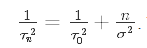
This can be written in terms of precisions as

這可以用精度來表示為

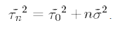
In this form we can clearly see that the posterior precision is the sum of the prior precision and the sample precision multiplied by the sample size. We can also re-write the posterior mean in terms of precisions:

在這種形式下，我們可以清楚地看到后驗精度是先驗精度與樣本精度的和乘以樣本大小。 我們還可以根據精度重寫后驗均值：

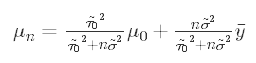
Here, we can clearly see that the posterior mean is a weighted average of the prior mean and sample mean.

在這里，我們可以清楚地看到后驗均值是先驗均值和樣本均值的加權平均值。

For our data, the posterior parameters are:

對于我們的數據，后驗參數為：

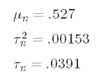
And there we have them — our updated parameters. Our posterior estimate for the average growth rate is about 52.7% — a decent bit lower than our sample average, but not overwhelmingly lower. We’ve taken a subjective belief, represented that belief with a distribution, and used that distribution to augment our analysis. Hooray! This is the power of Bayesian inference. As long as we can define our beliefs, we can incorporate them in a rigorous way in our analysis. Let’s talk a little more about what we have and also what we don’t have.

有了它們-我們更新的參數。 我們對平均增長率的后驗估計約為52.7％，雖然比我們的樣本平均值低了很多，但絕不算低。 我們采用了主觀信念，用分布表示了該信念，并使用該分布來擴大我們的分析。 萬歲！ 這就是貝葉斯推理的力量。 只要我們能夠定義我們的信念，我們就可以將其嚴格地納入我們的分析中。 讓我們再談一些關于我們擁有和不擁有的東西。

With our posterior standard deviation, we can compute a credible interval for our estimate. For those new to Bayesian statistics, a credible interval is not the same thing as a confidence interval even though they are computed in a similar manner. Our 95% credible interval for the posterior mean is .527+/?2?.0391.527+/?2?.0391 which leads to points of 44.88% and 60.52%. With this credible interval, we’re making the statement that we’re 95% sure that the true value of the posterior mean falls within the interval. Even at this point, we don’t treat this updated mean as a known entity. Furthermore, we are not saying that 52.7% is our forecast for revenue growth rate over the next rolling one-year period. If we wanted to make a forecast within this framework, we’d use the posterior predictive distribution. Since that is a separate topic, I won’t touch on it here, but the process of deriving that distribution is similar to deriving the posterior distribution.

利用我們的后驗標準差，我們可以計算出可信的區間。 對于貝葉斯統計新手來說，可信區間與置信區間并不相同，即使它們是以類似方式計算的。 我們的后驗平均值的95％可信區間為.527 +/- 2 * .0391.527 + /-/ 2 * .0391，得出的分數分別為44.88％和60.52％。 在此可信區間內，我們聲明95％的后驗均值的真實值落在該區間內。 即使在這一點上，我們也不會將這種更新的均值視為已知實體。 此外，我們并不是說52.7％是我們對下一個滾動的一年期內收入增長率的預測。 如果我們想在此框架內進行預測，則可以使用后驗預測分布。 由于這是一個單獨的主題，因此在此不再贅述，但是推導該分布的過程類似于推導后驗分布。

Two key implications should be noted from this analysis: the first is that as sample size grows larger, the posterior mean and posterior variance are more and more determined by the sample data. I’m not going to state that there’s an explicit cutoff, but at some amount of data, adding a prior doesn’t move the needle much all else equal. Intuitively, this is reasonable. If you have rich enough sampling data, the sampling data likely represents the actual structure in the data, and you may not see the need to utilize a prior distribution.

此分析應注意兩個關鍵含義：首先是隨著樣本量的增加，后均值和后方差越來越多地由樣本數據決定。 我不會說有一個明確的界限，但是在一定數量的數據下，添加一個先驗不會使其他所有條件都變差。 憑直覺，這是合理的。 如果您有足夠豐富的采樣數據，則采樣數據可能表示數據中的實際結構，并且您可能看不到需要利用先驗分布。

To emphasize the first point, we can re-run our analysis using strictly the year-end data which would leave us with a sample size of five data points. Using the same prior distribution, our new sampling mean and variance are about 59.8% and .012 (or 11.1% standard deviation), and our posterior mean and variance are 23% and .0019 (or 4.45% standard deviation). This posterior estimate for the mean is much lower than what we saw in our first iteration; with our sample size cut significantly, the prior plays a much heavier role in the output. The standard deviation didn’t change as much, but we can see that it’s larger even though our sampling standard deviation was smaller the second time around. We have a much lower estimate, and we have slightly less confidence in the estimate (wider credible interval).

為了強調第一點，我們可以嚴格使用年終數據來重新運行分析，這將使我們擁有五個數據點的樣本量。 使用相同的先驗分布，我們的新采樣均值和方差分別為59.8％和.012(或11.1％標準偏差)，而后驗均值和方差分別為23％和.0019(或4.45％標準偏差)。 該均值的后驗估計值比我們在第一次迭代中看到的要低得多。 由于我們的樣本量大大減少，因此先驗數據在輸出中起著舉足輕重的作用。 標準偏差變化不大，但是即使第二次采樣標準偏差較小，我們也可以看到它更大。 我們的估算值要低得多，而我們對估算值的信心則稍差(可信區間更大)。

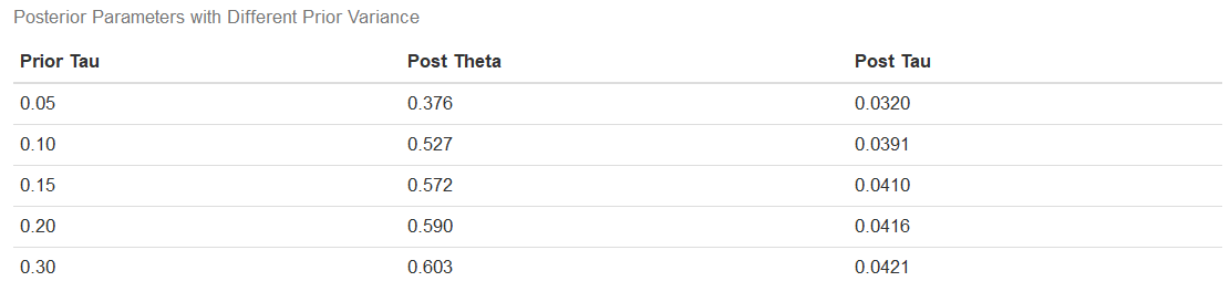
The second implication of our analysis is that the smaller the prior variance, the greater the prior precision and the greater impact it has on both the posterior mean and posterior variance. The more confidence we have in our prior, the more it will affect our posterior estimates. To illustrate this point, I re-ran our original analysis with different values for the prior variance. The values for the prior mean are all .045, and the sampling mean and variance come from our rolling revenue data. The table below shows the results of this experiment.

我們的分析的第二個含義是，先驗方差越小，先驗精度越高，它對后均值和后方方差的影響越大。 我們對先驗的信心越高，對后驗估計的影響就越大。 為了說明這一點，我使用先前的方差的不同值重新運行了我們的原始分析。 先前均值均為0.045，而抽樣均值和方差來自我們的滾動收入數據。 下表顯示了該實驗的結果。

I’ll also plot the distributions.

我還將繪制分布。

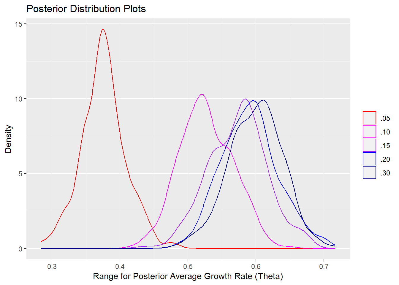
Notice how much closer to the prior mean our posterior distribution with prior variance set to .05 is. As we increase our prior variance (effectively signifying less confidence in the prior mean), the center of our posterior distribution moves closer to the sample mean. Also, while the magnitude of the changes in the posterior variances may not appear that great in the table, from the distribution plots above, we can see how the distributions get progressively wider; in other words, the credible interval for the true value of average growth widens.

注意，先驗方差設置為.05的后驗分布離先驗均值有多近。 隨著我們增加先驗方差(有效地表示對先驗均值的置信度降低)，我們后驗分布的中心移近樣本均值。 同樣，盡管后驗方差變化的幅度在表格中可能看起來不太大，但從上面的分布圖來看，我們可以看到分布如何逐漸變寬。 換句話說，平均增長真實值的可信區間變寬了。

摘要 (Summary)

Just to recap, we were analyzing a young company and wanted to estimate the true growth rate of its revenue. Given the small amount of sample data we had and a subjective belief that the average growth rate will be less than what the sample data suggests, we used Bayesian inference to augment our analysis. We defined a sampling model for our data, defined a prior for the average growth rate that reflected our subjective view, and utilized the normal-normal model to arrive at a posterior estimate and interval for the company’s average growth rate. I hope you found this brief introduction to Bayesian inference as well as the analysis of the results useful. I don’t recommend using the specific numbers in this piece for any valuation of MongoDB, but hopefully you can apply the concepts to your own analysis. I’m attaching a link to the GitHub repository for the code; nothing is particularly complicated, but I’ll share it in the spirit of transparency and reproducibility.

回顧一下，我們正在分析一家年輕的公司，并希望估計其收入的真實增長率。 考慮到我們擁有的樣本數據量很少，并且主觀認為平均增長率將低于樣本數據表明的速度，因此我們使用貝葉斯推斷來增強我們的分析。 我們為數據定義了一個采樣模型，為反映我們主觀觀點的平均增長率定義了先驗，并利用正常-正常模型得出了公司平均增長率的后驗估計和區間。 我希望您對貝葉斯推理的簡要介紹以及對結果的分析有用。 對于MongoDB的任何評估，我不建議使用本文中的特定數字，但希望您可以將這些概念應用于您自己的分析。 我正在將代碼的鏈接附加到GitHub存儲庫； 沒有什么特別復雜，但是我將本著透明和可復制的精神來分享。

https://github.com/vinai-oddiraju/TDS_Blog_Post1.git

https://github.com/vinai-oddiraju/TDS_Blog_Post1.git

Lastly, I want to thank the friends and family members who took time to read my drafts and provide feedback throughout the process. As this is my first time writing about a project in this manner, their support is especially appreciated. Thanks, and take care!

最后，我要感謝花時間閱讀我的草稿并在整個過程中提供反饋的朋友和家人。 由于這是我第一次以此方式撰寫項目，因此特別感謝他們的支持。 謝謝，保重！

免責聲明 (Disclaimer)

The thoughts and views expressed in this report are mine alone and do not necessarily reflect the views of my firm. This report is intended to be educational in nature and should not be construed as individual investment advice nor as a recommendation to buy, sell, or hold any security or to adopt any investment strategy.

本報告中表達的思想和觀點僅屬于我個人，不一定反映我公司的觀點。 本報告本質上是具有教育意義的報告，不應解釋為個人投資建議，也不能解釋為購買，出售或持有任何證券或采用任何投資策略的建議。

資料來源 (Sources)

[1] Hoff, Peter D. A First Course in Bayesian Statistical Methods (2007). Print.

[1] Hoff，PeterD。 貝葉斯統計方法的第一門課程 (2007年)。 打印。