P (tPYTHON)

Logical comparisons are used everywhere.

邏輯比較隨處可見 。

The Pandas library gives you a lot of different ways that you can compare a DataFrame or Series to other Pandas objects, lists, scalar values, and more. The traditional comparison operators (<, >, <=, >=, ==, !=) can be used to compare a DataFrame to another set of values.

Pandas庫為您提供了許多不同的方式，您可以將DataFrame或Series與其他Pandas對象，列表，標量值等進行比較。 傳統的比較運算符( <, >, <=, >=, ==, != )可用于將DataFrame與另一組值進行比較。

However, you can also use wrappers for more flexibility in your logical comparison operations. These wrappers allow you to specify the axis for comparison, so you can choose to perform the comparison at the row or column level. Also, if you are working with a MultiIndex, you may specify which index you want to work with.

但是，還可以使用包裝器在邏輯比較操作中提供更大的靈活性。 這些包裝器允許您指定要進行比較的軸 ，因此您可以選擇在行或列級別執行比較。 另外，如果您使用的是MultiIndex，則可以指定要使用的索引 。

In this piece, we’ll first take a quick look at logical comparisons with the standard operators. After that, we’ll go through five different examples of how you can use these logical comparison wrappers to process and better understand your data.

在本文中，我們將首先快速了解與標準運算符的邏輯比較。 之后，我們將介紹五個不同的示例，說明如何使用這些邏輯比較包裝器來處理和更好地理解您的數據。

The data used in this piece is sourced from Yahoo Finance. We’ll be using a subset of Tesla stock price data. Run the code below if you want to follow along. (And if you’re curious as to the function I used to get the data scroll to the very bottom and click on the first link.)

本文中使用的數據來自Yahoo Finance。 我們將使用特斯拉股價數據的子集。 如果要繼續，請運行下面的代碼。 (如果您對我用來使數據滾動到最底部并單擊第一個鏈接的功能感到好奇)。

import pandas as pd# fixed data so sample data will stay the same
df = pd.read_html("https://finance.yahoo.com/quote/TSLA/history?period1=1277942400&period2=1594857600&interval=1d&filter=history&frequency=1d")[0]df = df.head(10) # only work with the first 10 points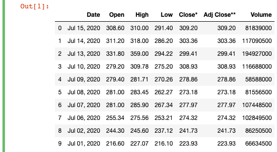

與熊貓的邏輯比較 (Logical Comparisons With Pandas)

The wrappers available for use are:

可用的包裝器有：

• eq (equivalent to ==) — equals to

  eq (等于== )—等于

• ne (equivalent to !=) — not equals to

  ne (等于!= )-不等于

• le (equivalent to <=) — less than or equals to

  le (等于<= )-小于或等于

• lt (equivalent to <) — less than

  lt (等于< )-小于

• ge (equivalent to >=) — greater than or equals to

  ge (等于>= )-大于或等于

• gt (equivalent to >) — greater than

  gt (等于> )-大于

Before we dive into the wrappers, let’s quickly review how to perform a logical comparison in Pandas.

在深入探討包裝之前，讓我們快速回顧一下如何在Pandas中進行邏輯比較。

With the regular comparison operators, a basic example of comparing a DataFrame column to an integer would look like this:

使用常規比較運算符，將DataFrame列與整數進行比較的基本示例如下所示：

old = df['Open'] >= 270

Here, we’re looking to see whether each value in the “Open” column is greater than or equal to the fixed integer “270”. However, if you try to run this, at first it won’t work.

在這里，我們正在查看“ Open”列中的每個值是否大于或等于固定整數“ 270”。 但是，如果嘗試運行此命令，則一開始它將無法工作。

You’ll most likely see this:

您很可能會看到以下內容：

TypeError: '>=' not supported between instances of 'str' and 'int'

TypeError: '>=' not supported between instances of 'str' and 'int'

This is important to take care of now because when you use both the regular comparison operators and the wrappers, you’ll need to make sure that you are actually able to compare the two elements. Remember to do something like the following in your pre-processing, not just for these exercises, but in general when you’re analyzing data:

這一點現在很重要，因為當您同時使用常規比較運算符和包裝器時，需要確保您確實能夠比較這兩個元素。 請記住，在預處理過程中，不僅要針對這些練習，而且在分析數據時通常要執行以下操作：

df = df.astype({"Open":'float',
                "High":'float',
                "Low":'float',
                "Close*":'float',
                "Adj Close**":'float',
                "Volume":'float'})

Now, if you run the original comparison again, you’ll get this series back:

現在，如果再次運行原始比較，您將獲得以下系列：

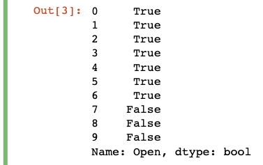
You can see that the operation returns a series of Boolean values. If you check the original DataFrame, you’ll see that there should be a corresponding “True” or “False” for each row where the value was greater than or equal to (>=) 270 or not.

您可以看到該操作返回了一系列布爾值。 如果檢查原始DataFrame，您會發現值大于或等于( >= )270的每一行都應該有一個對應的“ True”或“ False”。

Now, let’s dive into how you can do the same and more with the wrappers.

現在，讓我們深入研究如何使用包裝器做同樣的事情。

1.比較兩列的不平等 (1. Comparing two columns for inequality)

In the data set, you’ll see that there is a “Close*” column and an “Adj Close**” column. The Adjusted Close price is altered to reflect potential dividends and splits, whereas the Close price is only adjusted for splits. To see if these events may have happened, we can do a basic test to see if values in the two columns are not equal.

在數據集中，您將看到有一個“ Close *”列和一個“ Adj Close **”列。 調整后的收盤價被更改以反映潛在的股息和分割，而收盤價僅針對分割進行調整。 要查看是否可能發生了這些事件，我們可以進行基本測試以查看兩列中的值是否不相等。

To do so, we run the following:

為此，我們運行以下命令：

# is the adj close different from the close?
df['Close Comparison'] = df['Adj Close**'].ne(df['Close*'])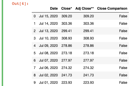

Here, all we did is call the .ne() function on the “Adj Close**” column and pass “Close*”, the column we want to compare, as an argument to the function.

在這里，我們.ne()在“ Adj Close **”列上調用.ne()函數，并傳遞“ Close *”(我們要比較的列)作為該函數的參數。

If we take a look at the resulting DataFrame, you’ll see that we‘ve created a new column “Close Comparison” that will show “True” if the two original Close columns are different and “False” if they are the same. In this case, you can see that the values for “Close*” and “Adj Close**” on every row are the same, so the “Close Comparison” only has “False” values. Technically, this would mean that we could remove the “Adj Close**” column, at least for this subset of data, since it only contains duplicate values to the “Close*” column.

如果我們看一下生成的DataFrame，您會看到我們創建了一個新列“ Close Compare”，如果兩個原始的Close列不同，則顯示“ True”，如果相同，則顯示“ False”。 在這種情況下，您可以看到每行上“ Close *”和“ Adj Close **”的值相同，因此“ Close Compare”只有“ False”值。 從技術上講，這意味著我們至少可以刪除此數據子集的“ Adj Close **”列，因為它僅包含“ Close *”列的重復值。

2.檢查一列是否大于另一列 (2. Checking if one column is greater than another)

We’d often like to see whether a stock’s price increased by the end of the day. One way to do this would be to see a “True” value if the “Close*” price was greater than the “Open” price or “False” otherwise.

我們經常想看看一天結束時股票的價格是否上漲了。 一種方法是，如果“收盤價”大于“開盤價”，則查看“真”值，否則查看“假”價。

To implement this, we run the following:

為了實現這一點，我們運行以下命令：

# is the close greater than the open?
df['Bool Price Increase'] = df['Close*'].gt(df['Open'])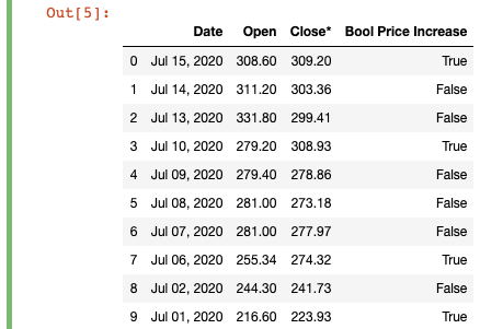

Here, we see that the “Close*” price at the end of the day was higher than the “Open” price at the beginning of the day 4/10 times in the first two weeks of July 2020. This might not be that informative because it’s such a small sample, but if you were to extend this to months or even years of data, it could indicate the overall trend of the stock (up or down).

在這里，我們看到，在2020年7月的前兩周，一天結束時的“收盤價”比一天開始時的“開盤價”高出4/10倍。因為這是一個很小的樣本，但是如果您將其擴展到數月甚至數年的數據，則可能表明存量的總體趨勢(上升或下降)。

3.檢查列是否大于標量值 (3. Checking if a column is greater than a scalar value)

So far, we’ve just been comparing columns to one another. You can also use the logical operators to compare values in a column to a scalar value like an integer. For example, let’s say that if the volume traded per day is greater than or equal to 100 million, we’ll call it a “High Volume” day.

到目前為止，我們只是在相互比較列。 您還可以使用邏輯運算符將列中的值與標量值(例如整數)進行比較。 例如，假設每天的交易量大于或等于1億，我們將其稱為“高交易量”日。

To do so, we run the following:

為此，我們運行以下命令：

# was the volume greater than 100m?
df['High Volume'] = df['Volume'].ge(100000000)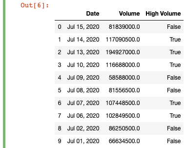

Instead of passing a column to the logical comparison function, this time we simply have to pass our scalar value “100000000”.

這次我們不必將列傳遞給邏輯比較函數，而只需傳遞標量值“ 100000000”。

Now, we can see that on 5/10 days the volume was greater than or equal to 100 million.

現在，我們可以看到5/10天的交易量大于或等于1億。

4.檢查列是否大于自身 (4. Checking if a column is greater than itself)

Earlier, we compared if the “Open” and “Close*” value in each row were different. It would be cool if instead, we compared the value of a column to the preceding value, to track an increase or decrease over time. Doing this means we can check if the “Close*” value for July 15 was greater than the value for July 14.

之前，我們比較了每行中的“打開”和“關閉*”值是否不同。 相反，如果我們將列的值與先前的值進行比較，以跟蹤隨時間的增加或減少，那將很酷。 這樣做意味著我們可以檢查7月15日的“ Close *”值是否大于7月14日的值。

To do so, we run the following:

為此，我們運行以下命令：

# was the close greater than yesterday's close?
df['Close (t-1)'] = df['Close*'].shift(-1)
df['Bool Over Time Increase'] = df['Close*'].gt(df['Close*'].shift(-1))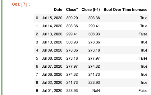

For illustration purposes, I included the “Close (t-1)” column so you can compare each row directly. In practice, you don’t need to add an entirely new column, as all we’re doing is passing the “Close*” column again into the logical operator, but we’re also calling shift(-1) on it to move all the values “up by one”.

為了便于說明，我在“ Close(t-1)”列中添加了一個標題，以便您可以直接比較每一行。 實際上，您不需要添加全新的列，因為我們要做的只是將“ Close *”列再次傳遞到邏輯運算符中，但是我們還對其調用了shift(-1)來進行移動所有值“加一”。

What’s going on here is basically subtracting one from the index, so the value for July 14 moves “up”, which lets us compare it to the real value on July 15. As a result, you can see that on 7/10 days the “Close*” value was greater than the “Close*” value on the day before.

這里發生的基本上是從索引中減去1，因此7月14日的值“向上”移動，這使我們可以將其與7月15日的實際值進行比較。結果，您可以看到在7/10天“關閉*”值大于前一天的“關閉*”值。

5.比較列與列表 (5. Comparing a column to a list)

As a final exercise, let’s say that we developed a model to predict the stock prices for 10 days. We’ll store those predictions in a list, then compare the both the “Open” and “Close*” values of each day to the list values.

作為最后的練習，假設我們開發了一個模型來預測10天的股價。 我們將這些預測存儲在列表中，然后將每天的“打開”和“關閉*”值與列表值進行比較。

To do so, we run the following:

為此，我們運行以下命令：

# did the open and close price match the predictions?
predictions = [309.2, 303.36, 300, 489, 391, 445, 402.84, 274.32, 410, 223.93]
df2 = df[['Open','Close*']].eq(predictions, axis='index')

Here, we’ve compared our generated list of predictions for the daily stock prices and compared it to the “Close*” column. To do so, we pass “predictions” into the eq() function and set axis='index'. By default, the comparison wrappers have axis='columns', but in this case, we actually want to work with each row in each column.

在這里，我們比較了生成的每日股票價格預測列表，并將其與“收盤價*”列進行了比較。 為此，我們將“預測”傳遞給eq()函數并設置axis='index' 。 默認情況下，比較包裝器具有axis='columns' ，但是在這種情況下，我們實際上要處理每一列中的每一行。

What this means is Pandas will compare “309.2”, which is the first element in the list, to the first values of “Open” and “Close*”. Then it will move on to the second value in the list and the second values of the DataFrame and so on. Remember that the index of a list and a DataFrame both start at 0, so you would look at “308.6” and “309.2” respectively for the first DataFrame column values (scroll back up if you want to double-check the results).

這意味著熊貓將把列表中的第一個元素“ 309.2”與“打開”和“關閉*”的第一個值進行比較。 然后它將移至列表中的第二個值和DataFrame的第二個值，依此類推。 請記住，列表的索引和DataFrame的索引都從0開始，因此對于第一個DataFrame列值，您將分別查看“ 308.6”和“ 309.2”(如果要仔細檢查結果，請向上滾動)。

Based on these arbitrary predictions, you can see that there were no matches between the “Open” column values and the list of predictions. There were 4/10 matches between the “Close*” column values and the list of predictions.

根據這些任意的預測，您可以看到“ Open”列值和預測列表之間沒有匹配項。 “ Close *”列值和預測列表之間有4/10個匹配項。

I hope you found this very basic introduction to logical comparisons in Pandas using the wrappers useful. Remember to only compare data that can be compared (i.e. don’t try to compare a string to a float) and manually double-check the results to make sure your calculations are producing the intended results.

我希望您發現使用包裝程序對熊貓進行邏輯比較非常基礎的介紹很有用。 請記住僅比較可以比較的數據(即不要嘗試將字符串與浮點數進行比較)，并手動仔細檢查結果以確保您的計算產生了預期的結果。

Go forth and compare!

繼續比較吧！

More by me:- 2 Easy Ways to Get Tables From a Website
- Top 4 Repositories on GitHub to Learn Pandas
- An Introduction to the Cohort Analysis With Tableau
- How to Quickly Create and Unpack Lists with Pandas
- Learning to Forecast With Tableau in 5 Minutes Or Less