pyspark上的動手推薦系統 (Hands-on recommender system on pyspark)

Recommender System is an information filtering tool that seeks to predict which product a user will like, and based on that, recommends a few products to the users. For example, Amazon can recommend new shopping items to buy, Netflix can recommend new movies to watch, and Google can recommend news that a user might be interested in. The two widely used approaches for building a recommender system are the content-based filtering (CBF) and collaborative filtering (CF).

推薦系統是一種信息過濾工具，旨在預測用戶喜歡的產品，并在此基礎上向用戶推薦一些產品。 例如，Amazon可以推薦要購買的新購物商品，Netflix可以推薦要觀看的新電影，而Google可以推薦用戶可能感興趣的新聞。構建推薦系統的兩種廣泛使用的方法是基于內容的過濾( CBF)和協作過濾(CF)。

To understand the concept of recommender systems, let us look at an example. The below table shows the user-item utility matrix Y where the value Rui denotes how item i has been rated by user u on a scale of 1–5. The missing entries (shown by ? in Table) are the items that have not been rated by the respective user.

為了理解推薦系統的概念，讓我們看一個例子。 下表顯示了用戶項效用矩陣 Y，其中Rui值表示用戶i如何以1-5的等級對項i進行評分。 缺少的條目(在表中用？顯示)是尚未由相應用戶評分的項目。

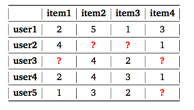
The objective of the recommender system is to predict the ratings for these items. Then the highest rated items can be recommended to the respective users. In real world problems, the utility matrix is expected to be very sparse, as each user only encounters a small fraction of items among the vast pool of options available. The code for this project can be found here.

推薦系統的目的是預測這些項目的評級。 然后可以向各個用戶推薦評分最高的項目。 在現實世界中，效用矩陣非常稀疏，因為每個用戶在大量可用選項中僅??會遇到一小部分項目。 該項目的代碼可以在這里找到。

顯式與隱式評級 (Explicit v.s. Implicit ratings)

There are two ways to gather user preference data to recommend items, the first method is to ask for explicit ratings from a user, typically on a concrete rating scale (such as rating a movie from one to five stars) making it easier to make extrapolations from data to predict future ratings. However, the drawback with explicit data is that it puts the responsibility of data collection on the user, who may not want to take time to enter ratings. On the other hand, implicit data is easy to collect in large quantities without any extra effort on the part of the user. Unfortunately, it is much more difficult to work with.

有兩種收集用戶偏好數據以推薦項目的方法，第一種方法是要求用戶提供明確的評分 ，通常以具體的評分標準(例如，將電影從一星評為五星)，使推斷更容易從數據中預測未來的收視率。 但是，顯式數據的缺點是將數據收集的責任交給了用戶，而用戶可能不想花時間輸入評分。 另一方面， 隱式數據易于大量收集，而無需用戶付出任何額外的努力。 不幸的是，要處理它要困難得多。

數據稀疏和冷啟動 (Data Sparsity and Cold Start)

In real world problems, the utility matrix is expected to be very sparse, as each user only encounters a small fraction of items among the vast pool of options available. Cold-Start problem can arise during addition of a new user or a new item where both do not have history in terms of ratings. Sparsity can be calculated using the below function.

在現實世界中，效用矩陣非常稀疏，因為每個用戶在大量可用選項中僅??會遇到一小部分項目。 在添加新用戶或新項目時，如果兩者都沒有評級歷史記錄，則會出現冷啟動問題。 稀疏度可以使用以下函數計算。

def get_mat_sparsity(ratings):# Count the total number of ratings in the datasetcount_nonzero = ratings.select("rating").count()# Count the number of distinct userIds and distinct movieIdstotal_elements = ratings.select("userId").distinct().count() * ratings.select("movieId").distinct().count()# Divide the numerator by the denominatorsparsity = (1.0 - (count_nonzero *1.0)/total_elements)*100print("The ratings dataframe is ", "%.2f" % sparsity + "% sparse.")get_mat_sparsity(ratings)

1.具有顯式評分的數據集(MovieLens) (1. Dataset with Explicit Ratings (MovieLens))

MovieLens is a recommender system and virtual community website that recommends movies for its users to watch, based on their film preferences using collaborative filtering. MovieLens 100M datatset is taken from the MovieLens website, which customizes user recommendation based on the ratings given by the user. To understand the concept of recommendation system better, we will work with this dataset. This dataset can be downloaded from here.

MovieLens是一個推薦器系統和虛擬社區網站，它基于用戶使用協作篩選的電影偏好來推薦電影供用戶觀看。 MovieLens 100M數據集來自MovieLens網站，該網站根據用戶給出的等級來自定義用戶推薦。 為了更好地理解推薦系統的概念，我們將使用此數據集。 可以從此處下載該數據集。

There are 2 tuples, movies and ratings which contains variables such as MovieID::Genre::Title and UserID::MovieID::Rating::Timestamp respectively.

有2個元組，電影和等級，其中分別包含MovieID :: Genre :: Title和UserID :: MovieID :: Rating :: Timestamp等變量。

Let’s load the data and explore the data. To load the data as a spark dataframe, import pyspark and instantiate a spark session.

讓我們加載數據并瀏覽數據。 要將數據加載為spark數據框，請導入pyspark并實例化spark會話。

from pyspark.sql import SparkSession
spark = SparkSession.builder.appName('Recommendations').getOrCreate()movies = spark.read.csv("movies.csv",header=True)
ratings = spark.read.csv("ratings.csv",header=True)
ratings.show()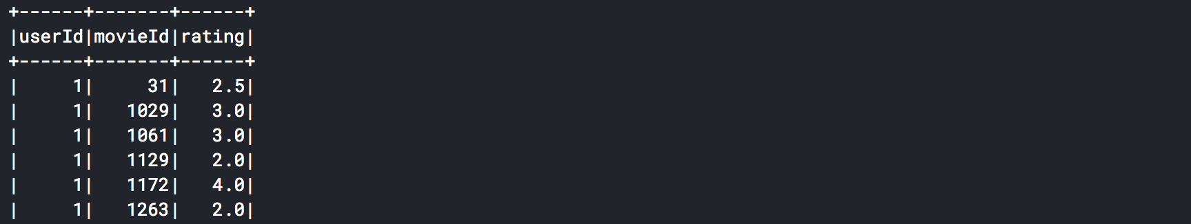

# Join both the data frames to add movie data into ratings
movie_ratings = ratings.join(movies, ['movieId'], 'left')
movie_ratings.show()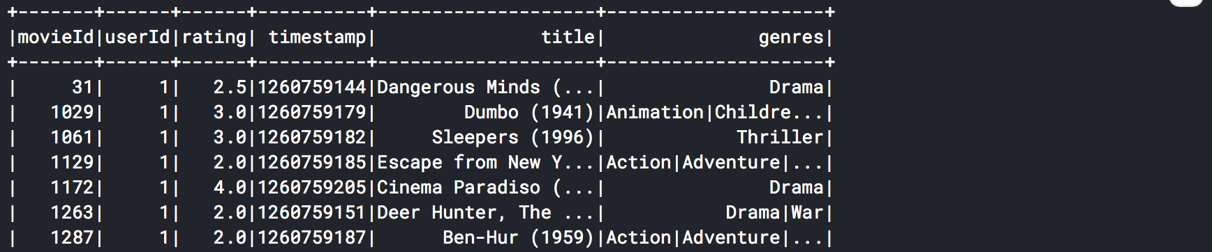

Let's calculate the data sparsity to understand the sparsity of the data. Please function that we built in the beginning of this article to get the sparsity. The movie lens data is 98.36% sparse.

讓我們計算數據稀疏度以了解數據稀疏度。 請使用我們在本文開頭構建的函數來獲得稀疏性。 電影鏡頭數據為98.36％稀疏。

get_mat_sparsity(ratings)

Before moving into recommendations, split the dataset into train and test. Please set the seed to reproduce results. We will look at different recommendation techniques in detail in the below sections.

在提出建議之前，請將數據集分為訓練和測試。 請設置種子以重現結果。 我們將在以下各節中詳細介紹不同的推薦技術。

# Create test and train set
(train, test) = ratings.randomSplit([0.8, 0.2], seed = 2020)

2.具有二進制等級的數據集(MovieLens) (2. Dataset with Binary Ratings (MovieLens))

With some datasets, we don’t have the luxury to work with explicit ratings. For those datasets we must infer ratings from the given information. In MovieLens dataset, let us add implicit ratings using explicit ratings by adding 1 for watched and 0 for not watched. We aim the model to give high predictions for movies watched.

對于某些數據集，我們沒有足夠的精力來使用明確的評分。 對于這些數據集，我們必須根據給定的信息推斷等級。 在MovieLens數據集中，讓我們使用顯式評級添加隱式評級，方法是將觀看次數增加1，將未觀看次數增加0。 我們的模型旨在為觀看的電影提供較高的預測。

Please note this is not the right dataset for implict ratings since there may be movies in the not watched set, which the user has actually watched but not given a rating.

請注意，這不是隱式收視率的正確數據集，因為可能有未觀看集中的電影，這些電影是用戶實際看過但未給出收視率的。

def get_binary_data(ratings):ratings = ratings.withColumn('binary', fn.lit(1))userIds = ratings.select("userId").distinct()movieIds = ratings.select("movieId").distinct()user_movie = userIds.crossJoin(movieIds).join(ratings, ['userId', 'movieId'], "left")user_movie = user_movie.select(['userId', 'movieId', 'binary']).fillna(0)return user_movieuser_movie = get_binary_data(ratings)

user_movie.show()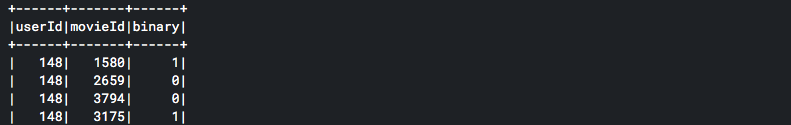

推薦方法 (Approaches to Recommendation)

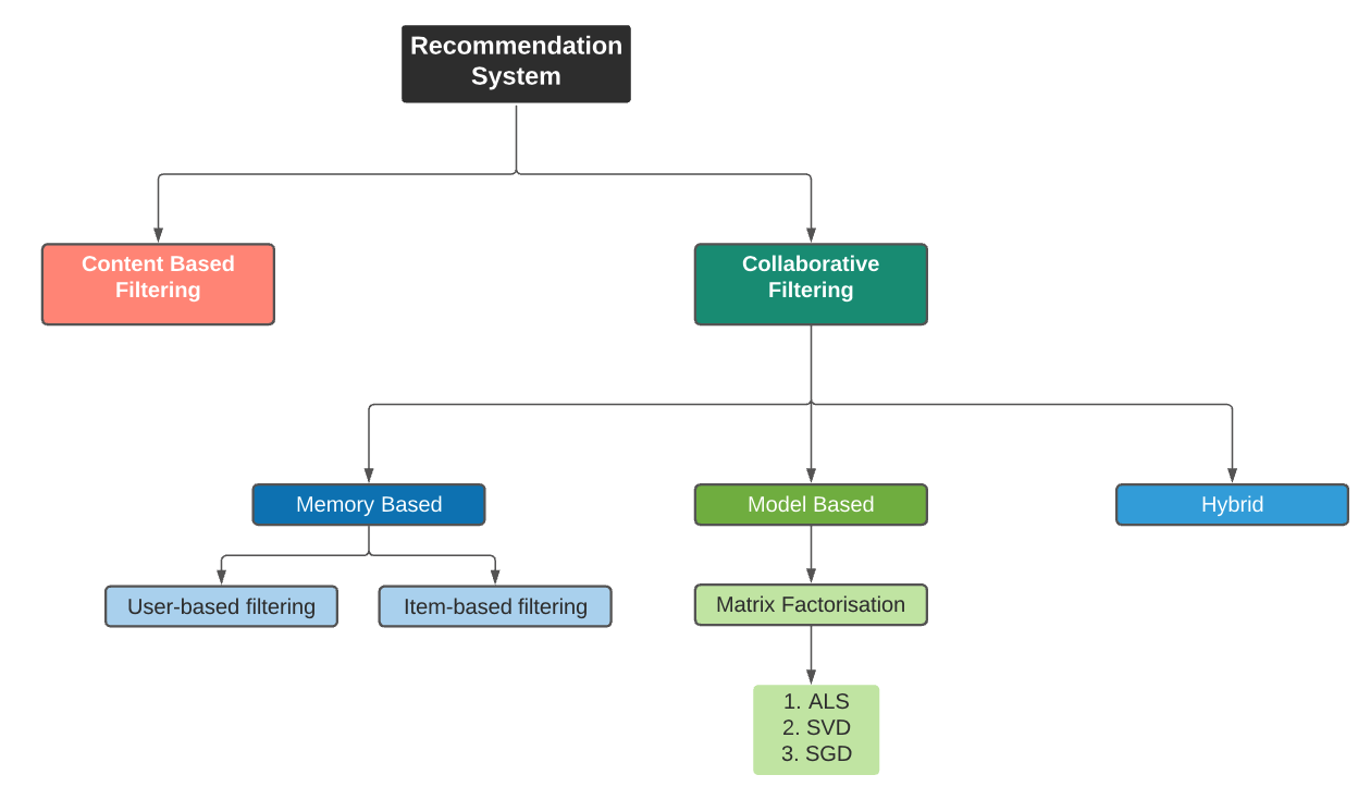
The two widely used approaches for building a recommender system are the content-based filtering (CBF) and collaborative filtering (CF), of which CBF is the most widely used.

建立推薦系統的兩種廣泛使用的方法是基于內容的過濾(CBF)和協作過濾(CF)，其中CBF的使用最為廣泛。

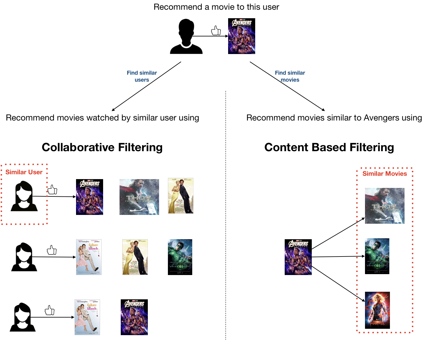
The below figure illustrates the concepts of CF and CBF. The primary difference between these two approaches is that CF looks for similar users to recommend items while CBF looks for similar contents to recommend items.

下圖說明了CF和CBF的概念。 這兩種方法之間的主要區別在于，CF尋找相似的用戶來推薦商品，而CBF尋找相似的內容來推薦商品。

協同過濾(CF) (Collaborative filtering (CF))

Collaborative filtering aggregates the past behaviour of all users. It recommends items to a user based on the items liked by another set of users whose likes (and dislikes) are similar to the user under consideration. This approach is also called the user-user based CF.

協同過濾匯總了所有用戶的過去行為。 它基于喜歡(和不喜歡)與正在考慮的用戶相似的另一組用戶喜歡的項目，向用戶推薦項目。 這種方法也稱為基于用戶-用戶的CF。

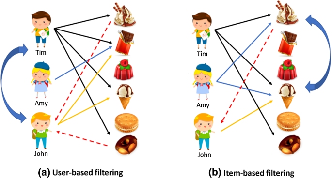
item-item based CF became popular later, where to recommend an item to a user, the similarity between items liked by the user and other items are calculated. The user-user CF and item-item CF can be achieved by two different ways, memory-based (neighbourhood approach) and model-based (latent factor model approach).

基于項目的CF后來變得很流行，向用戶推薦項目，計算用戶喜歡的項目與其他項目之間的相似度。 用戶-用戶CF和項目CF可以通過兩種不同的方式來實現，分別是基于內存的 (鄰域方法)和基于模型的 (潛在因子模型方法)。

1.基于內存的(鄰域方法) (1. The memory-based (neighbourhood approach))

To recommend items to user u1 in the user-user based neighborhood approach first a set of users whose likes and dislikes similar to the useru1 is found using a similarity metrics which captures the intuition that sim(u1, u2) >sim(u1, u3) where user u1 and u2 are similar and user u1 and u3 are dissimilar. similar user is called the neighbourhood of user u1.

為了在基于用戶-用戶的鄰域方法中向用戶u1推薦商品，首先使用相似度度量來發現一組用戶，這些用戶的相似之處和不相似之處類似于useru1，該相似度捕捉了sim(u1，u2)> sim(u1，u3)的直覺。 )，其中用戶u1和u2是相似的，而用戶u1和u3是不相似的。 類似的用戶稱為用戶u1的鄰居。

Neighbourhood approaches are most effective at detecting very localized relationships (neighbours), ignoring other users. But the downsides are that, first, the data gets sparse which hinders scalability, and second, they perform poorly in terms of reducing the RMSE (root-mean-squared-error) compared to other complex methods.

鄰域方法最有效地檢測非常本地化的關系(鄰域)，而忽略其他用戶。 但是缺點是，首先，數據稀疏，這阻礙了可伸縮性，其次，與其他復雜方法相比，它們在降低RMSE(均方根誤差)方面表現不佳。

2.基于模型(潛在因子模型方法) (2. The model-based (latent factor model approach))

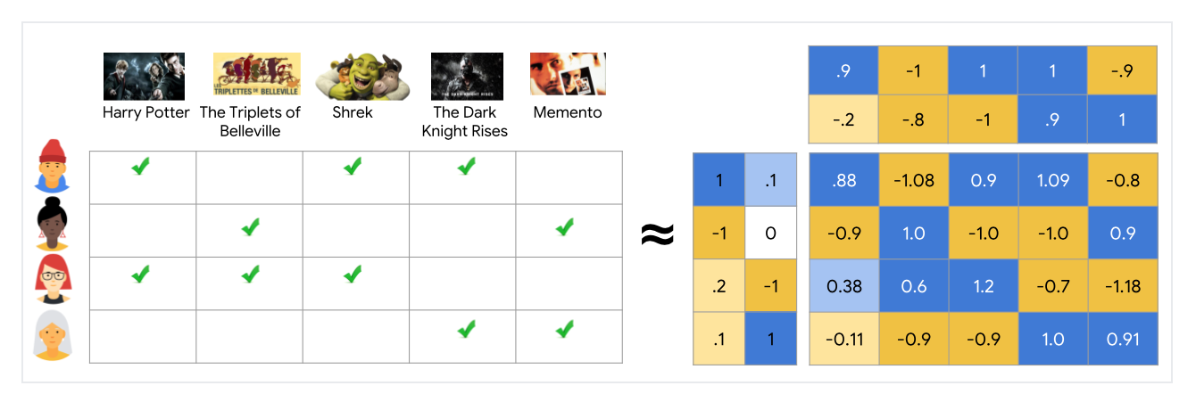
Latent factor model based collaborative filtering learns the (latent) user and item profiles (both of dimension K) through matrix factorization by minimizing the RMSE (Root Mean Square Error) between the available ratings yand their predicted values y?. Here each item i is associated with a latent (feature) vector xi, each user u is associated with a latent (profile) vector theta(u), and the rating y?(ui) is expressed as

基于潛在因子模型的協同過濾通過最小化可用評級y和其預測值y?之間的RMSE(均方根誤差)，通過矩陣分解來學習(潛在)用戶和項目配置文件(均為K維)。 在這里，每個項目i與一個潛在(特征)向量xi關聯，每個用戶u與一個潛在(特征)向量theta(u)關聯，并且等級y?(ui)表示為

Latent methods deliver prediction accuracy superior to other published CF techniques. It also addresses the sparsity issue faced with other neighbourhood models in CF. The memory efficiency and ease of implementation via gradient based matrix factorization model (SVD) have made this the method of choice within the Netflix Prize competition. However, the latent factor models are only effective at estimating the association between all items at once but fails to identify strong association among a small set of closely related items.

潛在方法提供的預測精度優于其他已發布的CF技術。 它還解決了CF中其他鄰域模型面臨的稀疏性問題。 通過基于梯度的矩陣分解模型(SVD)的存儲效率和易于實現的性能使其成為Netflix獎競賽中的首選方法。 但是，潛在因子模型僅可有效地一次估計所有項目之間的關聯，而無法識別少量緊密相關項目之間的強關聯。

建議使用交替最小二乘(ALS) (Recommendation using Alternating Least Squares (ALS))

Alternating Least Squares (ALS) matrix factorisation attempts to estimate the ratings matrix R as the product of two lower-rank matrices, X and Y, i.e. X * Yt = R. Typically these approximations are called ‘factor’ matrices. The general approach is iterative. During each iteration, one of the factor matrices is held constant, while the other is solved for using least squares. The newly-solved factor matrix is then held constant while solving for the other factor matrix.

交替最小二乘(ALS)矩陣分解嘗試將等級矩陣R估計為兩個較低等級的矩陣X和Y的乘積，即X * Yt =R。通常，這些近似值稱為“因子”矩陣。 一般方法是迭代的。 在每次迭代期間，因子矩陣之一保持恒定，而另一個因矩陣最小而求解。 然后，新求解的因子矩陣保持不變，同時求解其他因子矩陣。

In the below section we will instantiate an ALS model, run hyperparameter tuning, cross validation and fit the model.

在下面的部分中，我們將實例化ALS模型，運行超參數調整，交叉驗證并擬合模型。

1.建立一個ALS模型 (1. Build out an ALS model)

To build the model explicitly specify the columns. Set nonnegative as ‘True’, since we are looking at rating greater than 0. The model also gives an option to select implicit ratings. Since we are working with explicit ratings, set it to ‘False’.

要構建模型，請明確指定列。 將非負值設置為' True '，因為我們正在查看的評級大于0。該模型還提供了選擇隱式評級的選項。 由于我們正在使用顯式評級，因此請將其設置為“ False ”。

When using simple random splits as in Spark’s CrossValidator or TrainValidationSplit, it is actually very common to encounter users and/or items in the evaluation set that are not in the training set. By default, Spark assigns NaN predictions during ALSModel.transform when a user and/or item factor is not present in the model.We set cold start strategy to ‘drop’ to ensure we don’t get NaN evaluation metrics

當在Spark的CrossValidator或TrainValidationSplit使用簡單的隨機拆分時，遇到評估集中未包含的用戶和/或項目實際上很常見。 默認情況下，當模型中不存在用戶和/或項目因子時，Spark在ALSModel.transform期間分配NaN預測。 我們將冷啟動策略設置為“下降”，以確保沒有獲得NaN評估指標

# Import the required functions
from pyspark.ml.evaluation import RegressionEvaluator
from pyspark.ml.recommendation import ALS
from pyspark.ml.tuning import ParamGridBuilder, CrossValidator# Create ALS model
als = ALS(
         userCol="userId", 
         itemCol="movieId",
         ratingCol="rating", 
         nonnegative = True, 
         implicitPrefs = False,
         coldStartStrategy="drop"
)

2.超參數調整和交叉驗證 (2. Hyperparameter tuning and cross validation)

# Import the requisite packages
from pyspark.ml.tuning import ParamGridBuilder, CrossValidator
from pyspark.ml.evaluation import RegressionEvaluator

ParamGridBuilder: We will first define the tuning parameter using param_grid function, please feel free experiment with parameters for the grid. I have only chosen 4 parameters for each grid. This will result in 16 models for training.

ParamGridBuilder ：我們將首先使用param_grid函數定義調整參數，請隨意嘗試使用網格參數。 我只為每個網格選擇了4個參數。 這將產生16個訓練模型。

# Add hyperparameters and their respective values to param_grid
param_grid = ParamGridBuilder() \
            .addGrid(als.rank, [10, 50, 100, 150]) \
            .addGrid(als.regParam, [.01, .05, .1, .15]) \
            .build()

RegressionEvaluator: Then define the evaluator, select rmse as metricName in evaluator.

RegressionEvaluator ：然后定義評估器，在評估器中選擇rmse作為metricName。

# Define evaluator as RMSE and print length of evaluator
evaluator = RegressionEvaluator(
           metricName="rmse", 
           labelCol="rating", 
           predictionCol="prediction") 
print ("Num models to be tested: ", len(param_grid))

CrossValidator: Now feed both param_grid and evaluator into the crossvalidator including the ALS model. I have chosen number of folds as 5. Feel free to experiement with parameters.

CrossValidator ：現在將param_grid和Evaluator都輸入到包含ALS模型的crossvalidator中。 我選擇的折數為5。可以隨意使用參數進行實驗。

# Build cross validation using CrossValidator
cv = CrossValidator(estimator=als, estimatorParamMaps=param_grid, evaluator=evaluator, numFolds=5)

4.檢查最佳模型參數 (4. Check the best model parameters)

Let us check, which parameters out of the 16 parameters fed into the crossvalidator, resulted in the best model.

讓我們檢查一下輸入交叉驗證器的16個參數中的哪個參數產生了最佳模型。

print("**Best Model**")# Print "Rank"
print("  Rank:", best_model._java_obj.parent().getRank())# Print "MaxIter"
print("  MaxIter:", best_model._java_obj.parent().getMaxIter())# Print "RegParam"
print("  RegParam:", best_model._java_obj.parent().getRegParam())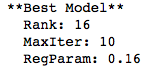

3.擬合最佳模型并評估預測 (3. Fit the best model and evaluate predictions)

Now fit the model and make predictions on test dataset. As discussed earlier, based on the range of parameters chosen we are testing 16 models, so this might take while.

現在擬合模型并對測試數據集進行預測。 如前所述，基于選擇的參數范圍，我們正在測試16個模型，因此這可能需要一段時間。

#Fit cross validator to the 'train' dataset
model = cv.fit(train)#Extract best model from the cv model above
best_model = model.bestModel# View the predictions
test_predictions = best_model.transform(test)RMSE = evaluator.evaluate(test_predictions)
print(RMSE)

The RMSE for the best model is 0.866 which means that on average the model predicts 0.866 above or below values of the original ratings matrix. Please note, matrix factorisation unravels patterns that humans cannot, therefore you can find ratings for a few users are a bit off in comparison to others.

最佳模型的RMSE為0.866，這意味著該模型平均預測比原始評級矩陣的值高或低0.866。 請注意，矩陣分解分解了人類無法做到的模式，因此您可以發現一些用戶的評分與其他用戶相比有些偏離。

4.提出建議 (4. Make Recommendations)

Lets go ahead and make recommendations based on our best model. recommendForAllUsers(n) function in als takes n recommedations. Lets go with 5 recommendations for all users.

讓我們繼續前進，并根據我們的最佳模型提出建議。 在als中的recommendedForAllUsers(n)函數需要n個建議。 讓我們為所有用戶提供5條建議。

# Generate n Recommendations for all users
recommendations = best_model.recommendForAllUsers(5)
recommendations.show()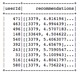

5.將建議轉換為可解釋的格式 (5. Convert recommendations into interpretable format)

The recommendations are generated in a format that easy to use in pyspark. As seen in the above the output, the recommendations are saved in an array format with movie id and ratings. To make these recommendations easy to read and compare t check if recommendations make sense, we will want to add more information like movie name and genre, then explode array to get rows with single recommendations.

推薦以易于在pyspark中使用的格式生成。 從上面的輸出中可以看到，推薦以帶有電影ID和等級的數組格式保存。 為了使這些建議易于閱讀和比較，并檢查建議是否有意義，我們將要添加更多信息，例如電影名稱和流派，然后爆炸數組以獲取包含單個建議的行。

nrecommendations = nrecommendations\
    .withColumn("rec_exp", explode("recommendations"))\
    .select('userId', col("rec_exp.movieId"), col("rec_exp.rating"))nrecommendations.limit(10).show()

這些建議有意義嗎？ (Do the recommendations make sense?)

To check if the recommendations make sense, join movie name and genre to the above table. Lets randomly pick 100th user to check if the recommendations make sense.

要檢查推薦的建議是否有意義，請將電影名稱和類型加入上表。 讓我們隨機選擇第100個用戶來檢查推薦是否有意義。

第100個用戶的ALS建議： (100th User’s ALS Recommendations:)

nrecommendations.join(movies, on='movieId').filter('userId = 100').show()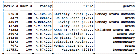

第100位使用者的實際偏好： (100th User’s Actual Preference:)

ratings.join(movies, on='movieId').filter('userId = 100').sort('rating', ascending=False).limit(10).show()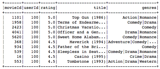

The movie recommended to the 100th user primarily belongs to comedy, drama, war and romance genres, and the movies preferred by the user as seen in the above table, match very closely with these genres.

推薦給第100位用戶的電影主要屬于喜劇，戲劇，戰爭和浪漫類，而上表中用戶偏愛的電影與這些流派非常匹配。

I hope you enjoyed reading. Please find the detailed codes in the Github Repository.

希望您喜歡閱讀。 請在Github存儲庫中找到詳細的代碼。