介紹 (Introduction)

One of the main applications of frequentist statistics is the comparison of sample means and variances between one or more groups, known as statistical hypothesis testing. A statistic is a summarized/compressed probability distribution; for example, the Gaussian distribution can be summarized with mean and standard deviation. In the view of a frequentist statistician, said statistics are random variables when estimated from data with unknown fixed true values behind them — and the question is whether groups are significantly different with respect to these estimated values.

頻度統計的主要應用之一是比較樣本均值和一個或多個組之間的方差 ，稱為統計假設檢驗 。 統計是匯總/壓縮的概率分布； 例如，可以用均值和標準差來概括高斯分布。 根據常客統計學家的觀點，當從其后具有未知固定真實值的數據進行估算時，所述統計信息是隨機變量 ，問題是，這些估算值的組是否顯著不同。

Suppose, for example, that a researcher is interested in the growth of children and wonders whether boys and girls of the same age, e.g. twelve years old, have the same height; said researcher collects a data set of the random variable height in some school. In this case, the randomness of height arises due to the sampled population (the children he finds that are twelve years old) and not necessarily due to noise — unless the measuring method is very inaccurate (this leads into the field of metrology). Different children from other schools would have led to different data.

例如，假設研究人員對兒童的成長感興趣，并且想知道同年齡(例如十二歲)的男孩和女孩的身高是否相同； 他說，研究人員在某所學校收集了一個隨機可變高度的數據集。 在這種情況下， 高度的隨機性是由于抽樣人口(他發現的十二歲的孩子)而不一定是由于噪聲引起的，除非測量方法非常不準確(這導致了計量領域)。 來自其他學校的不同孩子會得出不同的數據。

假設 (Hypothesis)

Assuming the research question is now formulated as “Do boys and girls of the same age have different heights?”, the first step would be to pose an hypothesis, although conventionally stated as null hypothesis (H0), i.e. boys and girls of the same age are the same height (there is no difference). This is analogous to thinking of two distributions for height with fixed mean μ and standard deviation σ generating the random variable height, however it is not known whether the means for boys (μ1) and girls (μ2) are the same. Additionally, there is an alternative hypothesis (HA) which is often the negation of the null hypothesis. The null hypothesis, in that case, would be

假設現在將研究問題表述為“同一年齡的男孩和女孩的身高不同嗎？”，第一步將是提出一個假設，盡管通常被稱為零假設 (H0) ，即相同年齡的男孩和女孩年齡是相同的身高(沒有差異)。 這類似于考慮具有固定均值μ和標準偏差σ的兩個高度分布生成隨機可變高度的想法，但是尚不清楚男孩( μ1 )和女孩( μ2 )的均值是否相同。 此外，還有一個替代假設(HA)，通常是對原假設的否定。 在這種情況下，原假設為

H0: μ1 = μ2

The researcher computes two sample means and might obtain some difference between them; but how can he be sure that this difference is true and not randomly unequal zero, as he could have also included other (or more) children in this study?

研究人員計算出兩個樣本均值，并且可能會在兩者之間獲得一些差異。 但是他如何確定這種差異是正確的，而不是隨機的不等于零，因為他也可以在本研究中包括其他(或更多)孩子？

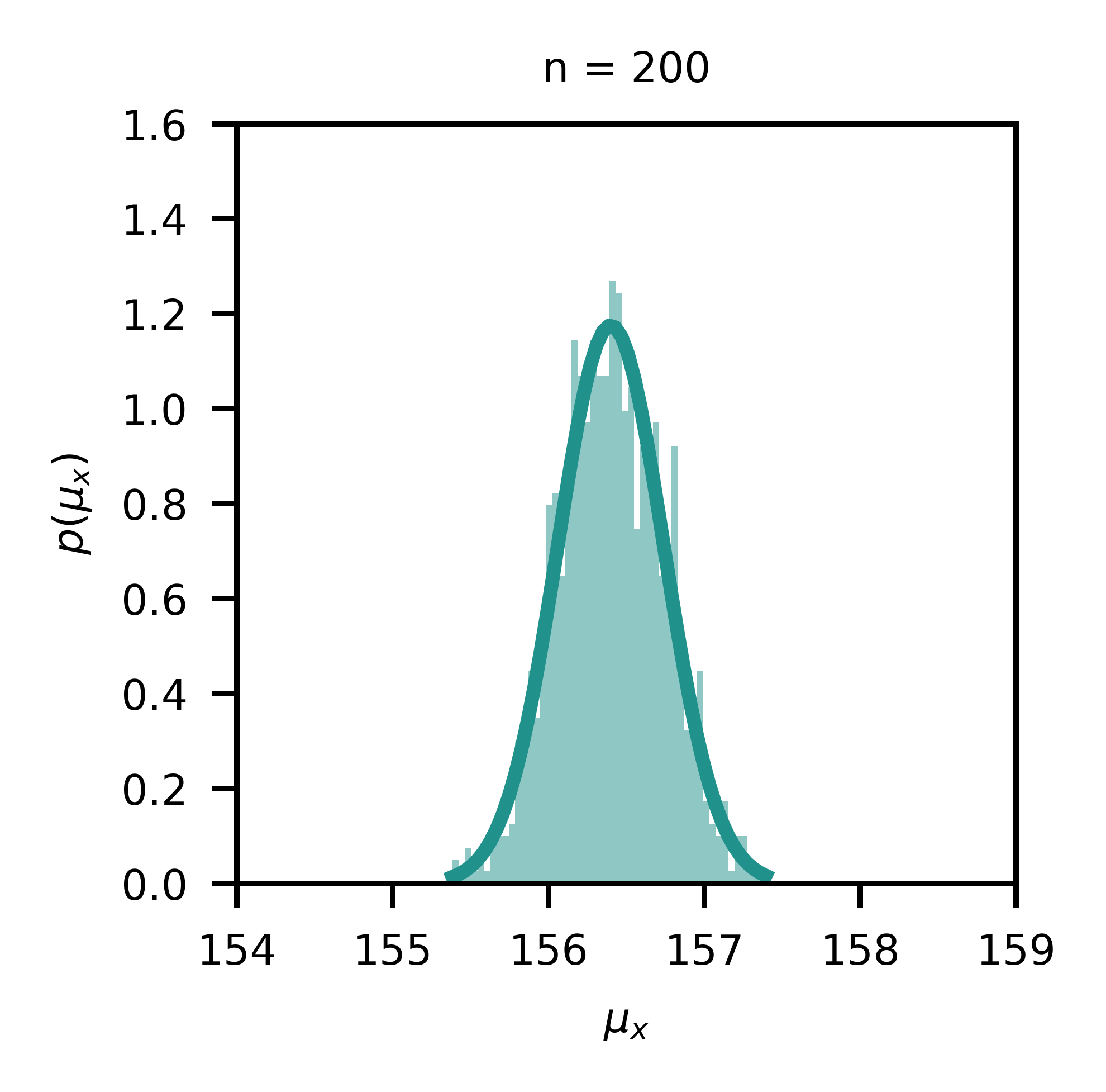
In Figure 1, a simulation with a random number generator is presented. Samples are drawn from a Gaussian distribution for a random variable x (e.g. height) with μ=156.4 and σ=4.8; in each subplot, n samples are drawn and the sample mean is computed; this process is repeated 1000 times for each sample size, and the corresponding histogram of sample means is visualized. This is essentially the distribution of sample means for different sample sizes, and it becomes evident that this distribution becomes narrower with increasing sample size as the standard deviation of the mean, also known as standard error (s.e.), scales with the inverse square root of the sample size.

在圖1中，展示了一個帶有隨機數生成器的仿真。 從高斯分布中抽取一個隨機變量x (例如height )的樣本，其中μ = 156.4和σ = 4.8； 在每個子圖中，繪制n個樣本并計算樣本均值； 對于每個樣本大小，此過程重復1000次，并顯示相應的樣本均值直方圖。 這實際上是不同樣本大小的樣本均值的分布，并且很明顯，隨著平均值的標準偏差(也稱為標準誤差)的增加，該分布會變窄 (se)，以樣本大小的平方根的倒數進行縮放。

s.e. = σ / sqrt(n)

置信區間 (Confidence Intervals)

The law of large numbers states that the average obtained from a large number of sampled random variables should be close to the expected value and will tend to become closer to the expected value as more samples are drawn. For example, for n=20, some sample means are 154 others are 160 — just by chance. Imagine computing two sample means, one for boys and one for girls; they could be different just by chance, particularly with higher probability in small sample sizes; the “true mean” can be located more precisely by the sample mean if enough samples are collected; but what if this is not the case? In many studies, the number of participants is often limited.

大數定律 指出從大量抽樣隨機變量獲得的平均值應該接近預期值，并且隨著抽取更多樣本，趨向于接近預期值。 例如，對于n = 20，一些樣本均值是154，其他樣本均值是160，這只是偶然。 想象一下計算兩個樣本均值，一個用于男孩，一個用于女孩； 它們可能只是偶然而不同，尤其是在小樣本量中更有可能； 如果收集了足夠的樣本，則可以通過樣本平均值更精確地定位“真實平均值”； 但是如果不是這種情況怎么辦？ 在許多研究中，參與者的數量通常是有限的。

This is the origin of the so-called confidence interval. A confidence interval for an estimated statistic is a random interval calculated from the sample that contains the true value with some specified probability. For example, a 95% confidence interval for the mean is a random interval that contains the true mean with probability of 0.95; if we were to take many random samples and compute a confidence interval for each one, about 95% of these intervals would contain the true mean. (The two concepts of randomness and frequency are ubiquitous in the frequentist’s paradigm.) This way, the distributions in Figure 1 can be approximated with confidence intervals. To compute a confidence interval, the quantiles z from the t-distribution corresponding to the chosen probability 1-α (e.g. α = 0.05 for 95%) are multiplied with the standard error, centered on the sample mean on both sides.

這就是所謂的置信區間的起源。 估計統計量的置信區間是從樣本中計算出的隨機區間，其中包含具有某個指定概率的真實值。 例如，均值的95％置信區間是包含真實均值且概率為0.95的隨機區間； 如果我們要抽取許多隨機樣本并為每個樣本計算一個置信區間，那么這些區間中的大約95％將包含真實均值。 (在頻率論者的范式中，隨機性和頻率這兩個概念無處不在。)這樣，圖1中的分布可以用置信區間來近似。 為了計算置信區間，將對應于所選概率1- α (例如，對于95％的α = 0.05)的t分布的分位數z與標準誤差相乘，并以兩側的樣本平均值為中心。

confidence interval = [μ - z(α/2)*s.e., μ + z(α/2)*s.e.]

The t-distribution is a continuous probability distribution that arises when estimating the sample mean of a normally distributed population in situations where the sample size is small and the population standard deviation is unknown — which is quite common. (The t-distribution will be discussed more in detail below.)

t分布是連續的概率分布，在樣本量較小且總體標準偏差未知的情況下估計正態分布總體的樣本均值時會出現這種概率分布，這很常見。 (t分布將在下面詳細討論。)

統計檢驗 (Statistical Tests)

It is of relevance to know the distribution of the random variable for the selection of the appropriate statistical test. More precisely, a parametric tests like the t-test assumes a normal distribution of the random variable, but this might not necessarily be the case. In that case, it might be reasonable to use a non-parametric test such as the Mann-Whitney U test. However, the Mann-Whitney U test uses another null hypothesis in which the probability distributions of both groups are related to each other

了解隨機變量的分布對于選擇適當的統計檢驗至關重要。 更準確地說，像t檢驗這樣的參數檢驗假設正態分布 隨機變量的大小，但不一定是這種情況。 在這種情況下，使用諸如Mann-Whitney U檢驗的非參數檢驗可能是合理的。 但是，Mann-Whitney U檢驗使用另一個無效假設，在該假設中兩組的概率分布相互關聯

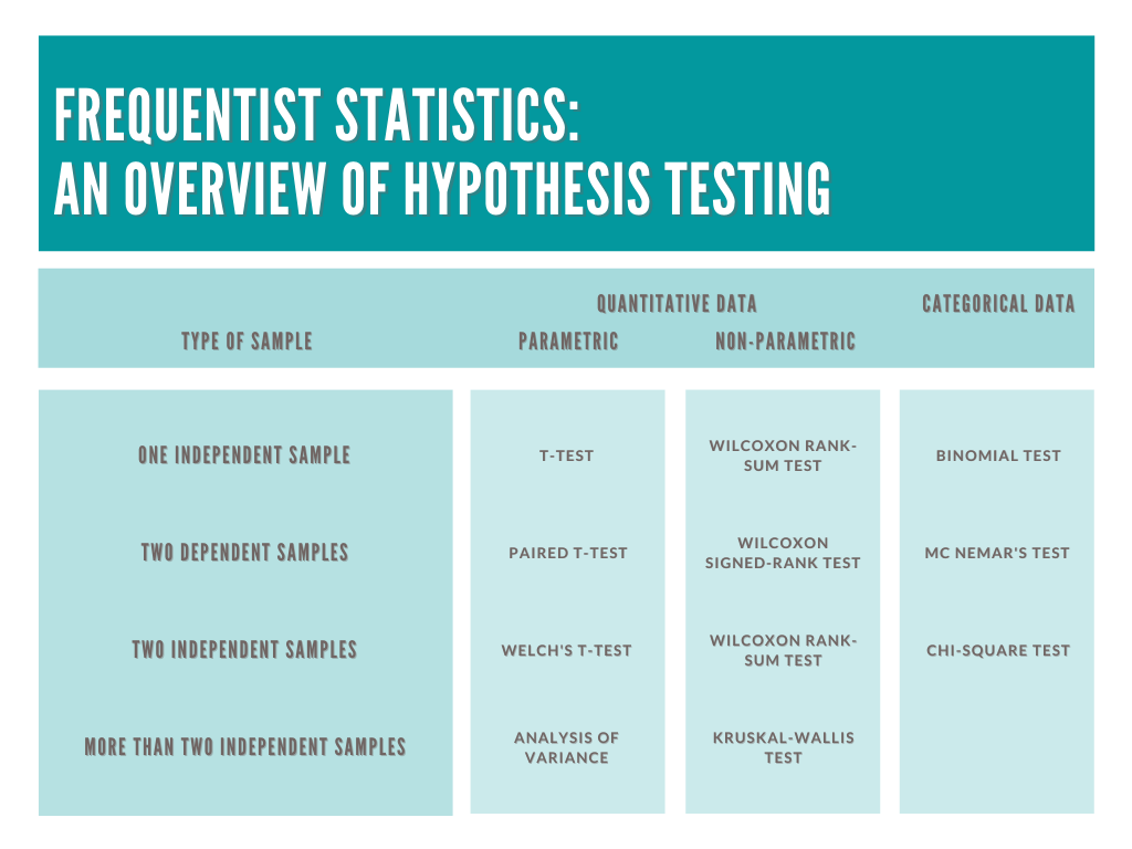
H0: p(height1) = p(height2)

There is a whole zoo of statistical tests (Figure 2); which test to use depends on the type of data (quantitative vs. categorical), whether the data is normally distributed (parametric vs. non-parametric), and whether samples are paired (independent vs. dependent). However, it is important to be aware the null hypothesis is not always the same, so the conclusions change slightly.

有一個完整的統計測試動物園(圖2)； 使用哪種測試取決于數據類型(定量與分類)，數據是否為正態分布(參數與非參數)以及樣本是否成對(獨立與依賴)。 但是，重要的是要知道零假設并不總是相同的，因此結論略有變化。

Once the assumptions are verified, a test is chosen, and the test statistic is computed from the two samples with sizes n and m. In this example, it would be the t-statistic T, which is distributed according to the t-distribution (with n+m-2 degrees of freedom). S is the pooled (aggregated) sample variance. In addition, it is worth mentioning that T scales with the sample size(s).

一旦驗證了假設，就選擇一個測試，然后從大小為n和m的兩個樣本中計算出測試統計量。 在這個例子中，它將是t統計量 T ，根據 t分布 ( n + m -2自由度)。 S是合并(匯總)的樣本方差。 另外，值得一提的是， T與樣本量成正比。

T = (mean(height1) - mean(height2)) / (sqrt(S) * (1/n + 1/m))S = ((n - 1) * std(height1) + (m - 1) * std(height1)) / (n + m - 2)

Note the similarity of the t-statistic to the z-score, which is associated with the Gaussian distribution. The higher the absolute value of the z-score the lower the probability, which is also true for the t-distribution. Hence, the higher the absolute value of the t-statistic, the less probable it is that the null hypothesis is true.

注意t統計量與z得分的相似性， 與高斯分布有關。 z分數的絕對值越高，概率越低，這對于t分布也是如此。 因此，t統計量的絕對值越高，原假設為真的可能性就越小。

Just to provide some clarification, the t-statistic follows a t-distribution because the standard deviation/error is unknown and has to be estimated from (little amount of) data. If it was known, one would use a normal distribution and the z-score. For larger sample sizes, the distribution of the t-statistic becomes more and more normal as the standard error approaches zero. (Note that the estimated standard deviation is also a random variable that follows a Chi-square distribution with n-1 degrees of freedom.)

只是為了澄清一下，t統計量遵循t分布，因為標準偏差/誤差是未知的，必須從(少量)數據中估算出來。 如果知道的話，將使用正態分布和z得分。 對于更大的樣本量，隨著標準誤差接近零，t統計量的分布變得越來越正態。 (請注意，估算的標準偏差也是遵循卡方分布的隨機變量 具有n-1個自由度。)

p值 (p-Value)

As mentioned above, statistical hypothesis testing deals with group comparison and the goal is to assess whether differences across groups are significant or not — given the estimated sample statistics. For this purpose, the sufficient statistics, their corresponding confidence intervals, and the p-value are computed. The p-value is the probability associated with the T-statistic using the t-distribution, similar as the probability associated to a z-score and the Gaussian distribution (Figure 3). In most cases, a two-sided test is applied in which the absolute value of the T-statistic is assessed. In mathematical terms, the p-value is

如上所述，統計假設檢驗用于組比較，目標是評估給定的樣本統計量，評估組之間的差異是否顯著。 為此，要計算足夠的統計量，其相應的置信區間和p值 。 p值是使用t分布與T統計量相關聯的概率，類似于與z得分和高斯分布相關的概率(圖3)。 在大多數情況下，將使用雙向檢驗來評估T統計量的絕對值。 用數學術語來說，p值是

p = 2*min{Pr(θ <= T|H0), Pr(θ >= T|H0)}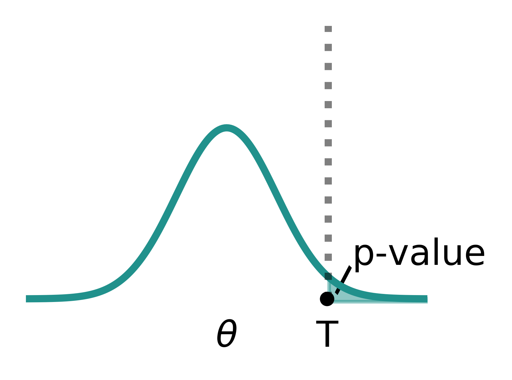

As such, the p-value is the largest probability of obtaining test results θ at least as “extreme” as the result actually observed T — under the assumption that the null hypothesis is true. A very small p-value means that such an “extreme” observed outcome is very unlikely under the null hypothesis (the observed data is “sufficiently” inconsistent with the null hypothesis).

這樣，p值獲得測試結果至少θ為“極端”作為實際觀察到T中的結果的最大概率-假設零假設為真下。 p值非常小意味著在原假設下觀察到的這種“極端”結果極不可能(觀察數據與原假設“足夠”不一致)。

假陽性和假陰性 (False Positive and False Negative)

If the p-value is lower than some threshold α, the difference is said to be statistically significant. Rejecting the null hypothesis when it is actually true is called a type I error (false positive), and the probability of a type I error is called the significance level (“some threshold”) α. Accepting the null hypothesis when it is false is called a type II error (false negative) and its probability is denoted by β. The probability, that the null hypothesis is rejected when it is false is called the power of the test and is equals 1-β. By being more strict with the significance level α, the risk for false positives can be minimized. However, tuning for false negatives is more difficult because the alternative hypothesis includes all other possibilities.

如果p值低于某個閾值α ，則該差異被認為具有統計學意義 。 在原假設為真時拒絕原假設的情況稱為I類錯誤 (假陽性)，而將I類錯誤的概率稱為顯著性水平(“某個閾值”) α 。 如果為假則接受原假設，稱為II型錯誤 (假否定) 其概率用β表示。 當零假設為假時拒絕原假設的概率稱為檢驗的功效，等于1- β 。 通過對顯著性水平α進行更嚴格的規定，可以將誤報的風險降到最低。 但是，由于其他假設包括所有其他可能性，因此調整假陰性更加困難。

In practice it is the case that the choice of α is essentially arbitrary; small values, such as 0.05 or even 0.01 are commonly used in science. One critisim of this approach is that the null hypothesis has to be rejected or accepted, although this would not be necessary; for instance, in a Bayesian approach, both hypotheses could exist simultaneously with some associated posterior probability (modeling the likelihood of hypotheses).

在實踐中， α的選擇基本上是任意的。 在科學中通常使用較小的值，例如0.05甚至0.01。 這種方法的一個罪魁禍首是原假設必須被拒絕或接受，盡管這不是必須的。 例如，在貝葉斯方法中，兩個假設可以同時存在一些相關的后驗概率(對假設的可能性進行建模)。

結束語 (Final Remarks)

It should be stated that there is a duality between confidence intervals and hypothesis tests. Without going too much into detail, it is worth mentioning that if two confidence intervals overlap for a given level α, the null hypothesis is rejected.

應該指出，置信區間和假設檢驗之間存在二重性。 無需贅述，值得一提的是，如果對于給定的水平α ，兩個置信區間重疊，則原假設被拒絕。

However, only because a difference is statistically significant, it might not be relevant. A small p-value can be observed for an effect that is not meaningful or important. In fact, the larger the sample sizes, the smaller the minimum effect needed to produce a statistically significant p-value.

但是，僅因為差異在統計上顯著，才可能不相關。 可以觀察到較小的p值，表示該效果沒有意義或不重要。 實際上，樣本數量越大，產生統計上顯著的p值所需的最小影響越小。

Lastly, the conclusions are worthless is they are based on wrong (e.g. biased) data. It is important to guarantee that sampled data is of high quality and whitout biases — which is not a trivial task at all.

最后，結論是毫無根據的，因為它們基于錯誤(例如有偏見)的數據。 重要的是要確保采樣數據的高質量和偏見 - 這根本不是一件簡單的任務。