數據分析 (DATA ANALYSIS)

Being a regular at a restaurant is great.

乙 eing定期在餐廳是偉大的。

When I started university, my dad told me I should find a restaurant I really liked and eat there every month with some friends. Becoming a regular was supposed to be great because you got to build personal connections with the staff and create a ton of good memories over time.

當我上大學時，父親告訴我應該找到我真正喜歡的餐廳，并每月和一些朋友在那兒吃飯。 成為普通人應該很棒，因為隨著時間的推移，您必須與員工建立個人聯系并創造大量美好的回憶。

But how much do regulars actually help businesses?

但是常客實際上對企業有多大幫助？

You might think that because the same people keep coming back to order, they would be the “customer group” that makes up a majority of the restaurant’s sales. However, this intuitive answer isn’t always the case. If you took a fast-food chain near a popular tourist attraction, it could be that the customer group of those who only ordered once contribute far more to sales than the locals who eat there every week.

您可能會認為，由于相同的人不斷恢復訂購，因此他們將成為構成餐廳銷售額絕大部分的“客戶群”。 但是，這種直觀答案并非總是如此。 如果您在一個受歡迎的旅游景點附近搭了一條快餐連鎖店，那可能是那些只訂購一次的顧客群對銷售的貢獻遠大于每周在那兒用餐的當地人。

To answer questions like these, we can turn to cohort analysis. This type of analytics focuses on breaking up the users or customers of a business (or service) into different groups. Members of a cohort will exhibit the same behavior in a specified time range. For example, customers who ordered again within a week after their first purchase could be the first cohort, then customers who ordered within two weeks would be the second cohort, and so on.

要回答此類問題，我們可以轉向隊列分析。 這種類型的分析重點在于將業務(或服務)的用戶或客戶分為不同的組。 同類群組成員在指定的時間范圍內將表現出相同的行為。 例如，在第一次購買后一周內再次訂購的客戶可能是第一批，然后在兩周內訂購的客戶將成為第二批，依此類推。

Cohort analysis can help you identify trends across a customer’s “life cycle” (the time over which they purchase your goods or use your service), so you can better understand how to serve each cohort. It’s one thing to know that you had 500 total users of your app in one month. It’s another to know that of those 500, only 12 were users of your app since its first launch. With that knowledge, then you could try to understand why those 12 kept using the app after its launch and try to improve your service based on those findings.

同類群組分析可以幫助您確定客戶“生命周期”(他們購買商品或使用服務的時間)內的趨勢，因此您可以更好地了解如何為每個同類群組提供服務。 知道您在一個月內擁有500個應用程序用戶是一回事。 另一個要知道的是，自您的應用首次發布以來，在這500個應用中，只有12個是該應用的用戶。 有了這些知識，您就可以嘗試了解為什么這12個應用在啟動后仍繼續使用該應用，并根據這些發現嘗試改善您的服務。

Now, let’s take a look at how you can perform this analysis with Tableau/

現在，讓我們看一下如何使用Tableau /

Tableau中同類群組分析的四個步驟 (Four steps to cohort analysis in Tableau)

There is no one-click “cohort analysis” option in Tableau, but you can create such a visualization with just a few quick steps.

Tableau中沒有一鍵式的“隊列分析”選項，但是您只需幾個簡單的步驟就可以創建這種可視化。

If you want to follow along, we’re going to be working with the “Sample — Superstore” data set that comes with Tableau. The main question we’re going to answer is as follows:

如果您想繼續學習，我們將使用Tableau隨附的“樣本-超級商店”數據集。 我們要回答的主要問題如下：

How much do longer-tenured customers impact total and annual profit of the business?

長期客戶會在多大程度上影響企業的總利潤和年利潤？

Here, we’ll be creating cohorts of customers grouped by the first year they placed an order with the business. We’ll look at how much each cohort has contributed to total profit, as well as how much each cohort contributed to the profit in each year.

在這里，我們將創建按客戶下訂單的第一年分組的客戶群。 我們將查看每個同類群組對總利潤的貢獻，以及每個同類群組每年對利潤的貢獻。

To do so, we’ll need to calculate the minimum order date for every customer. This might sound easy enough, as each order has a corresponding “Order Date”. However, to group customers by this calculated field, we’ll need to use a Level of Detail (LOD) expression in Tableau. We’ll specifically be using a FIXED LOD calculation so that we can give each customer its own “First Order Date” value.

為此，我們需要計算每個客戶的最短訂購日期。 這聽起來很容易，因為每個訂單都有一個對應的“訂單日期”。 但是，要按此計算字段對客戶進行分組，我們需要在T??ableau中使用Level of Detail (LOD)表達式。 我們將特別使用FIXED LOD計算，以便為每個客戶提供自己的“首次訂購日期”值。

Here’s how we would get the “First Order Date” field:

這是我們如何獲取“第一訂單日期”字段的方法：

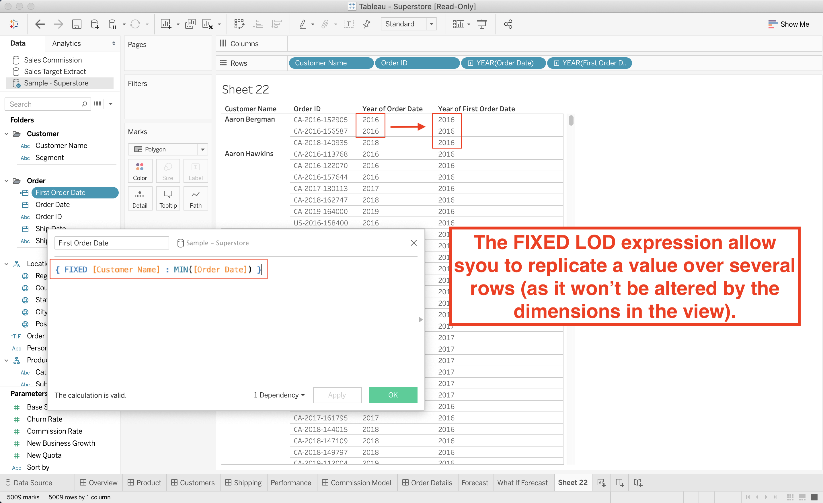
The calculated field is pretty simple:

計算字段非常簡單：

{FIXED [Customer Name] : MIN([Order Date]) }

{FIXED [Customer Name] : MIN([Order Date]) }

Here, we’re looking for the minimum order date for every customer and “fixing” it. If we were to only write MIN([Order Date]), we wouldn’t get the correct result when we create a graph without “Customer Name” in the field, as Tableau would then attempt to calculate the minimum order date for whatever other dimensions are in the field.

在這里，我們正在尋找每個客戶的最小訂購日期并“定下來”。 如果我們只寫MIN([Order Date]) ，則在我們創建的字段中沒有“ Customer Name”的圖形時，我們將無法獲得正確的結果，因為Tableau隨后將嘗試計算其他任何商品的最小訂購日期尺寸在字段中。

Now, to get our first graph with the total contribution of each customer cohort, there are just three steps:

現在，要獲得包含每個客戶群組的總貢獻的第一張圖，只需執行以下三個步驟：

1. Drag Profit and First Order Date into the view (or just double-click them). These should change to SUM([Profit]) and YEAR(First Order Date).

   將Profit和First Order Date拖到視圖中(或雙擊它們)。 這些應更改為SUM([Profit])和YEAR(First Order Date) 。

2. Click show me (or CTRL+Click/CMD+Click) and select the pie chart option.
   單擊“向我顯示”(或CTRL +單擊/ CMD +單擊)，然后選擇餅圖選項。

3. (Optional) resize the visualization to “Entire View”, add a Percent of Total calculation, and edit the “Label” to make the graph look prettier.

   (可選)將可視化文件的大小調整為“整個視圖”，添加“ Percent of Total計算，然后編輯“標簽”以使圖形看起來更漂亮。

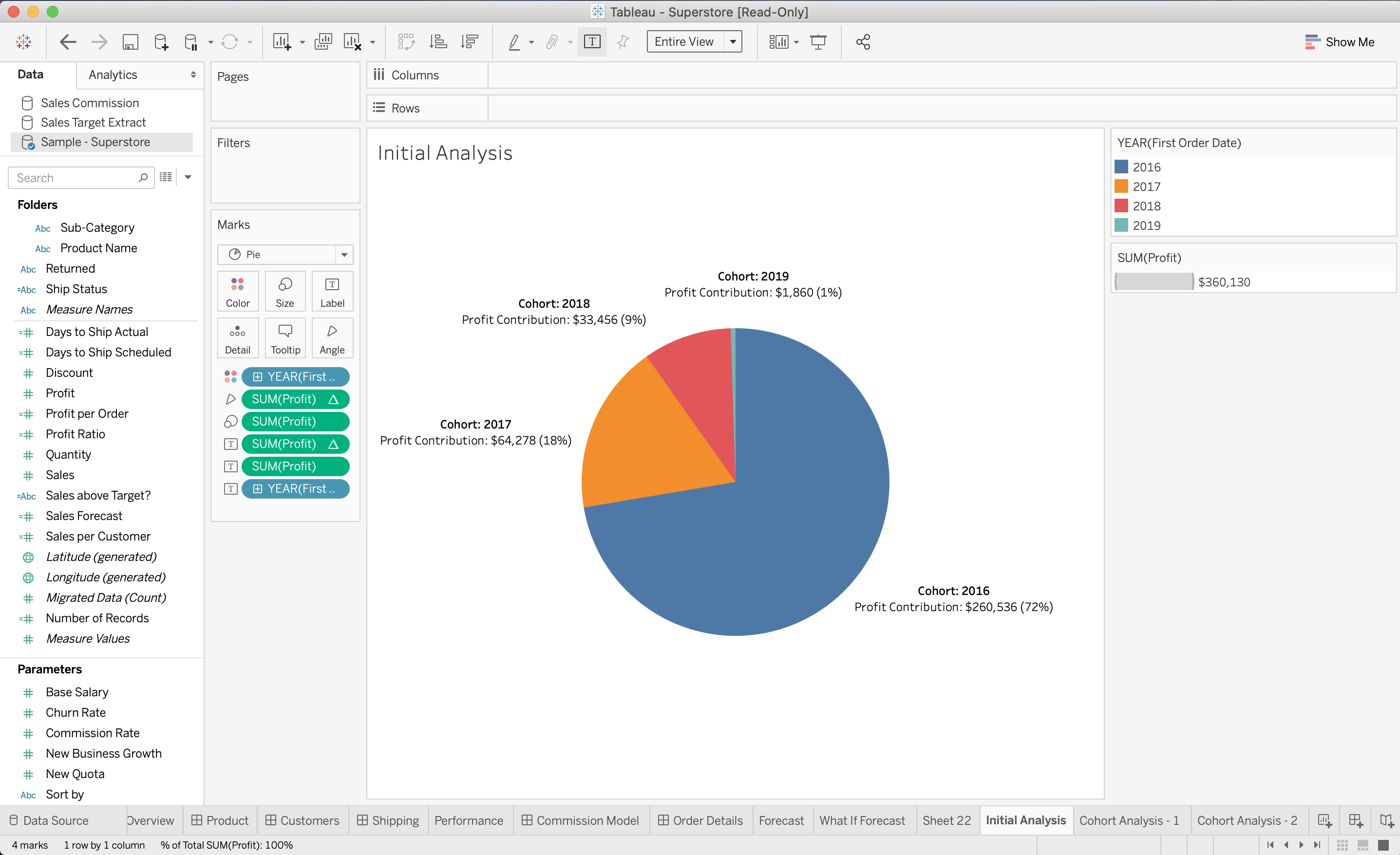
Ta-da!

-

Here, the sales are summed across all years the store has been in business. You can see that the majority of the profit came from the 2016 cohort, which is the first year the store was in business. It would be more interesting to see a chart with this data plotted across several years, so we could see if the 2016 cohort kept contributing a large percentage of yearly profit over time.

在這里，匯總了該商店營業的所有年份的銷售額。 您可以看到，大部分利潤來自2016年同期，這是該商店開業的第一年。 看到一個圖表，用多年的數據繪制圖表會更有趣，因此我們可以看到2016年同期是否隨著時間的推移繼續貢獻了很大一部分年度利潤。

To make our second graph with the yearly cohort profit contribution, we do the following steps:

為了使第二張圖表具有年度同類群組利潤貢獻，我們執行以下步驟：

1. Drag [Order Date] to “Columns” and [Profit] to “Rows”. These should change to YEAR(Order Date) and SUM([Profit]).

   將[Order Date]拖到“列”，將[Profit]拖到“行”。 這些應更改為YEAR(Order Date)和SUM([Profit]) 。

2. Drag [First Ordet Date] to the “Color” mark.

   將[First Ordet Date] “顏色”標記。

3. Click show me (or CTRL+Click/CMD+Click) and select the stacked bar chart option.
   單擊“向我顯示”(或CTRL +單擊/ CMD +單擊)，然后選擇堆積的條形圖選項。

4. (Optional) resize the visualization to “Entire View” and drag [Profit] to the “Label” mark.

   (可選)將可視化文件的大小調整為“整個視圖”，然后將[Profit]拖動到“標簽”標記。

Ta-da part 2!

Ta-da Part 2！

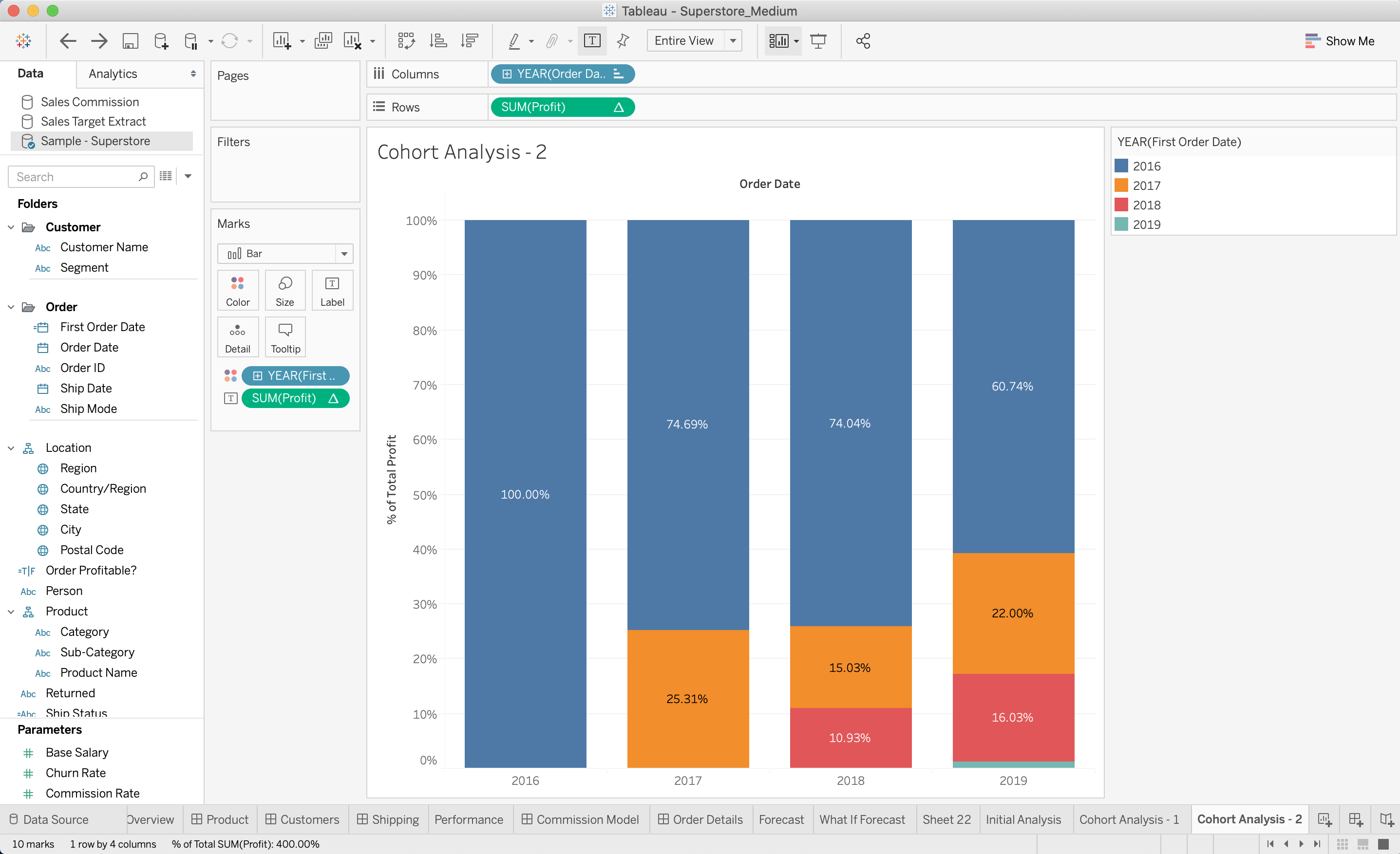
With this graph, we can see that over time a large amount of the yearly profit still comes from the 2016 cohort. This means that the customers who were with the business at the very beginning continue to purchase goods that give the business high profit, and we can even see that their absolute profit contribution increases every year (from $51,984 in 2016 to $91,600).

通過此圖，我們可以看到，隨著時間的流逝，大量的年度利潤仍然來自2016年同期。 這意味著從一開始就與公司打交道的客戶繼續購買可為公司帶來高利潤的商品，我們甚至可以看到他們的絕對利潤貢獻每年都在增加(從2016年的51,984美元增加到91,600美元)。

It’s also interesting that the 2017 cohort’s profit contribution actually decreased from 2017 to 2018. Perhaps the business spent a lot of money to acquire new customers, which then decreased the profit gained from sales to the 2017 cohort.

有趣的是，2017年隊列的利潤貢獻實際上從2017年減少到2018年。也許企業花了很多錢獲得新客戶，然后這減少了從2017年隊列的銷售獲得的利潤。

Another interesting visualization would be the same one as above, but with the yearly profit percentage contribution. To do so, follow these quick steps:

另一個有趣的可視化將與上面相同，但是具有年度利潤百分比貢獻。 為此，請按照以下快速步驟操作：

1. Duplicate the previous graph
   復制上一張圖

2. Right-click on SUM(Profit) and you’ll see the option to add a Quick Table Calculation. Select Percent of Total.

   右鍵單擊SUM(Profit) ，您將看到添加Quick Table Calculation的選項。 選擇Percent of Total 。

3. Right-click on SUM(Profit) again, select “Compute Using” and set it to “Table (down)”.

   再次右鍵單擊SUM(Profit) ，選擇“ Compute Using”，然后將其設置為“ Table(down)”。

Ta-da part 3!

Ta-da第3部分！

With this graph, we same the same numbers as before, but this time with the Y-axis set to Percentage. We can clearly see that over time, the majority of the profit comes from the 2016 cohort. It would be helpful to investigate why this is happening by analyzing the 2016 cohort for features that distinguish them from the other three. Doing so could help the business either better tailor its offerings to other customer cohorts, or it could choose to simply focus only on the 2016 cohort and maximize its profit that way.

在此圖表中，我們使用與以前相同的數字，但是這次Y軸設置為“百分比”。 我們可以清楚地看到，隨著時間的流逝，大部分利潤來自2016年同期。 通過分析2016年同類群組中有區別于其他三個類別的功能，有助于調查為什么會發生這種情況。 這樣做可以幫助企業更好地為其他客戶群體量身定制其產品，或者可以選擇僅專注于2016年客戶群體并以此最大化其利潤。

I hope you found this quick introduction to conducting a cohort analysis with Tableau useful! You can do a lot more with Tableau than just create the basic graphs from “Show Me”, but that means understanding some of its more advanced features like LOD Expressions. These and other skills can help you make sense of the data your business collects and drive well-informed decision making.

我希望您發現使用Tableau進行同類群組分析的快速入門對您有所幫助！ 使用Tableau可以做更多的事情，而不僅僅是從“ Show Me”中創建基本圖形，但這意味著了解其一些更高級的功能，例如LOD Expressions 。 這些技能和其他技能可以幫助您理解企業收集的數據并推動明智的決策。

If you’re looking to acquire a deeper understanding of Tableau, you may want to check out this comprehensive introduction to the Tableau Desktop Certifications.

如果您希望對Tableau有了更深入的了解，則可能需要查看有關Tableau Desktop認證的全面介紹 。

For a look at another type of analysis, you can do with Tableau, review this quick guide to forecasting.

要查看另一種類型的分析，可以使用Tableau，請查看此預測快速指南 。

Happy graphing.

快樂繪圖。