?? Note — This post is a part of Learning data analysis with python series. If you haven’t read the first post, some of the content won’t make sense. Check it out here.

Note? 注意 -這篇文章是使用python系列學習數據分析的一部分。 如果您還沒有閱讀第一篇文章，那么其中一些內容將毫無意義。 在這里查看 。

In the previous article, we talked about Pandas Series, working with real world data and handling missing values in data. Although series are very useful but most real world datasets contain multiple rows and columns and that’s why Dataframes are used much more than series. In this post, we’ll talk about dataframe and some operations that we can do on dataframe objects.

在上一篇文章中，我們討論了Pandas系列，它使用現實世界的數據并處理數據中的缺失值。 盡管序列非常有用，但是大多數現實世界的數據集都包含多個行和列，這就是為什么使用數據框比序列更多的原因。 在本文中，我們將討論數據框以及我們可以對數據框對象執行的一些操作。

什么是DataFrame？ (What is a DataFrame?)

As we saw in the previous post, A Series is a container of scalars,A DataFrame is a container for Series. It’s a dictionary like data structure for Series. A DataFrame is similar to a two-dimensional hetrogeneous tabular data(SQL table). A DataFrame is created using many different types of data such as dictionary of Series, dictionary of ndarrays/lists, a list of dictionary, etc. We’ll look at some of these methods to create a DataFrame object and then we’ll see some operations that we can apply on a DataFrame object to manipulate the data.

正如我們在上一篇文章中看到的，A Series是標量的容器，DataFrame是Series的容器。 這是一個字典，類似于Series的數據結構。 DataFrame類似于二維異構表格數據(SQL表)。 DataFrame是使用許多不同類型的數據創建的，例如Series字典，ndarrays / lists字典，字典列表等。我們將研究其中的一些方法來創建DataFrame對象，然后再看一些我們可以應用到DataFrame對象上的操作來操縱數據。

使用Series字典的DataFrame (DataFrame using dictionary of Series)

In[1]:
    d = {
    'col1' : pd.Series([1,2,3], index = ["row1", "row2", "row3"]),
    'col2' : pd.Series([4,5,6], index = ["row1", "row2", "row3"])
    }    df = pd.DataFrame(d)Out[1]:
        col1    col2
row1     1       4
row2     2       5
row3     3       6

As shown in above code, the keys of dict of Series becomes column names of the DataFrame and the index of the Series becomes the row name and all the data gets mapped by the row name i.e.,order of the index in the Series doesn’t matter.

如上面的代碼所示，Series的dict鍵成為DataFrame的列名，Series的索引成為行名，并且所有數據都按行名映射，即Series中索引的順序不物。

使用ndarrays / list的DataFrame (DataFrame using ndarrays/lists)

In[2]:
    d = {
        'one' : [1.,2.,3.],
        'two' : [4.,5.,6.]
    }    df = pd.DataFrame(d)Out[2]:
    one  two
0   1.0  4.0
1   2.0  5.0
2   3.0  6.0

As shown in the above code, when we use ndarrays/lists, if we don’t pass the index then the range(n) becomes the index of the DataFrame.And while using the ndarray to create a DataFrame, the length of these arrays must be same and if we pass an explicit index then the length of this index must also be of same length as the length of the arrays.

如上面的代碼所示，當我們使用ndarrays / lists時，如果不傳遞索引，則range(n)將成為DataFrame的索引。當使用ndarray創建DataFrame時，這些數組的長度必須相同，并且如果我們通過顯式索引，則該索引的長度也必須與數組的長度相同。

使用字典列表的DataFrame (DataFrame using list of dictionaries)

In[3]:
    d = [
        {'one': 1, 'two' : 2, 'three': 3},
        {'one': 10, 'two': 20, 'three': 30, 'four': 40}
    ]    df = pd.DataFrame(d)Out[3]:
    one two three four
0    1   2   3     NaN
1    10  20  30    40.0
In[4]:
    df = pd.DataFrame(d, index=["first", "second"])Out[4]:        one two three four
first    1   2   3     NaN
second   10  20  30    40.0

And finally, as described above we can create a DataFrame object using a list of dictionary and we can provide an explicit index in this method,too.

最后，如上所述，我們可以使用字典列表創建DataFrame對象，并且也可以在此方法中提供顯式索引。

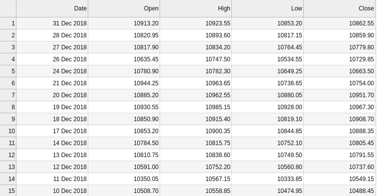
Although learning to create a DataFrame object using these methods is necessary but in real world, we won’t be using these methods to create a DataFrame but we’ll be using external data files to load data and manipulate that data. So, let’s take a look how to load a csv file and create a DataFrame.In the previous post, we worked with the Nifty50 data to demonstrate how Series works and similarly in this post, we’ll load Nifty50 2018 data, but in this dataset we have data of Open, Close, High and Low value of Nifty50. First let’s see what this dataset looks like and then we’ll load it into a DataFrame.

盡管學習使用這些方法創建DataFrame對象是必要的，但在現實世界中，我們不會使用這些方法來創建DataFrame，而是將使用外部數據文件加載數據并操縱該數據。 因此，讓我們看一下如何加載一個csv文件并創建一個DataFrame。在上一篇文章中，我們使用Nifty50數據來演示Series的工作原理，與此類似，在本文中，我們將加載Nifty50 2018數據，但是在本文中在數據集中，我們具有Nifty50的開盤價，收盤價，高價和低價的數據。 首先，讓我們看看該數據集的外觀，然后將其加載到DataFrame中。

In[5]:
    df = pd.read_csv('NIFTY50_2018.csv')Out[5]:
        Date      Open        High        Low        Close
0   31 Dec 2018  10913.20   10923.55    10853.20    10862.55
1   28 Dec 2018  10820.95   10893.60    10817.15    10859.90
2   27 Dec 2018  10817.90   10834.20    10764.45    10779.80
3   26 Dec 2018  10635.45   10747.50    10534.55    10729.85
4   24 Dec 2018  10780.90   10782.30    10649.25    10663.50
...     ...         ...        ...         ...         ...
241 05 Jan 2018  10534.25   10566.10    10520.10    10558.85
242 04 Jan 2018  10469.40   10513.00    10441.45    10504.80
243 03 Jan 2018  10482.65   10503.60    10429.55    10443.20
244 02 Jan 2018  10477.55   10495.20    10404.65    10442.20
245 01 Jan 2018  10531.70   10537.85    10423.10    10435.55In[6]:
    df = pd.read_csv('NIFTY50_2018.csv', index_col=0)Out[6]:
                  Open        High        Low        Close
    Date
31 Dec 2018     10913.20    10923.55    10853.20    10862.55
28 Dec 2018     10820.95    10893.60    10817.15    10859.90
27 Dec 2018     10817.90    10834.20    10764.45    10779.80
26 Dec 2018     10635.45    10747.50    10534.55    10729.85
24 Dec 2018     10780.90    10782.30    10649.25    10663.50
     ...           ...        ...         ...          ...
05 Jan 2018     10534.25    10566.10    10520.10    10558.85
04 Jan 2018     10469.40    10513.00    10441.45    10504.80
03 Jan 2018     10482.65    10503.60    10429.55    10443.20
02 Jan 2018     10477.55    10495.20    10404.65    10442.20
01 Jan 2018     10531.70    10537.85    10423.10    10435.55

As shown above, we have loaded the dataset and created a DataFrame called df and looking at the data, we can see that we can set the index of our DataFrame to the Date column and in the second cell we did that by providing the index_col parameter in the read_csv method.

如上所示，我們已經加載了數據集并創建了一個名為df的DataFrame并查看數據，我們可以看到可以將DataFrame的索引設置為Date列，在第二個單元格中，我們通過提供index_col參數來完成此操作在read_csv方法中。

There are many more parameters available in the read_csv method such as usecols using which we can deliberately ask the pandas to only load provided columns, na_values to provide explicit values that pandas should identify as null values and so on and so forth. Read more about all the parameters in pandas documentation.

read_csv方法中還有許多可用的參數，例如usecols ，我們可以使用這些參數故意要求熊貓僅加載提供的列，使用na_values提供熊貓應將其標識為空值的顯式值，依此類推。 在pandas 文檔中閱讀有關所有參數的更多信息。

Now, let’s look at some of the basic operations that we can perform on the dataframe object in order to learn more about our data.

現在，讓我們看一下可以對dataframe對象執行的一些基本操作，以了解有關數據的更多信息。

In[7]:
    # Shape(Number of rows and columns) of the DataFrame
    df.shapeOut[7]:
    (246,4)In[8]:
    # List of index
    df.indexOut[8]:
    Index(['31 Dec 2018', '28 Dec 2018', '27 Dec 2018', '26 Dec 2018',
       '24 Dec 2018', '21 Dec 2018', '20 Dec 2018', '19 Dec 2018',
       '18 Dec 2018', '17 Dec 2018',
       ...
       '12 Jan 2018', '11 Jan 2018', '10 Jan 2018', '09 Jan 2018',
       '08 Jan 2018', '05 Jan 2018', '04 Jan 2018', '03 Jan 2018',
       '02 Jan 2018', '01 Jan 2018'],
      dtype='object', name='Date', length=246)In[9]:
    # List of columns
    df.columnsOut[9]:
    Index(['Open', 'High', 'Low', 'Close'], dtype='object')In[10]:
    # Check if a DataFrame is empty or not
    df.emptyOut[10]:
    False

It’s very crucial to know data types of all the columns because sometimes due to corrupt data or missing data, pandas may identify numeric data as ‘object’ data-type which isn’t desired as numeric operations on the ‘object’ type of data is costlier in terms of time than on float64 or int64 i.e numeric datatypes.

了解所有列的數據類型非常關鍵，因為有時由于損壞的數據或缺少的數據，大熊貓可能會將數字數據標識為“對象”數據類型，這是不希望的，因為對“對象”類型的數據進行數字運算是在時間上比在float64或int64上更昂貴，即數值數據類型。

In[11]:
    # Datatypes of all the columns
    df.dtypesOut[11]:
    Open     float64
    High     float64
    Low      float64
    Close    float64
    dtype: object

We can use iloc and loc to index and get the particular data from our dataframe.

我們可以使用iloc和loc進行索引并從數據框中獲取特定數據。

In[12]:
    # Indexing using implicit index
    df.iloc[0]Out[12]:
    Open     10913.20
    High     10923.55
    Low      10853.20
    Close    10862.55
    Name: 31 Dec 2018, dtype: float64In[13]:
    # Indexing using explicit index
    df.loc["01 Jan 2018"]Out[13]:
    Open     10531.70
    High     10537.85
    Low      10423.10
    Close    10435.55
    Name: 01 Jan 2018, dtype: float64

We can also use both row and column to index and get specific cell from our dataframe.

我們還可以使用行和列來索引并從數據框中獲取特定的單元格。

In[14]:
    # Indexing using both the axes(rows and columns)
    df.loc["01 Jan 2018", "High"]Out[14]:
    10537.85

We can also perform all the math operations on a dataframe object same as we did on series.

我們也可以像處理序列一樣對數據框對象執行所有數學運算。

In[15]:
    # Basic math operations
    df.add(10)Out[15]:
                      Open        High        Low        Close
    Date
31 Dec 2018     10923.20    10933.55    10863.20    10872.55
28 Dec 2018     10830.95    10903.60    10827.15    10869.90
27 Dec 2018     10827.90    10844.20    10774.45    10789.80
26 Dec 2018     10645.45    10757.50    10544.55    10739.85
24 Dec 2018     10790.90    10792.30    10659.25    10673.50
     ...           ...        ...         ...          ...
05 Jan 2018     10544.25    10576.10    10530.10    10568.85
04 Jan 2018     10479.40    10523.00    10451.45    10514.80
03 Jan 2018     10492.65    10513.60    10439.55    10453.20
02 Jan 2018     10487.55    10505.20    10414.65    10452.20
01 Jan 2018     10541.70    10547.85    10433.10    10445.55

We can also aggregate the data using the agg method. For instance, we can get the mean and median values from all the columns in our data using this method as show below.

我們還可以使用agg方法匯總數據。 例如，可以使用此方法從數據中所有列獲取平均值和中值，如下所示。

In[16]:
    # Aggregate one or more operations
    df.agg(["mean", "median"])Out[16]:
            Open            High            Low            Close
mean    10758.260366    10801.753252    10695.351423    10749.392276
median  10704.100000    10749.850000    10638.100000    10693.000000

However, pandas provide a more convenient method to get a lot more than just minimum and maximum values across all the columns in our data. And that method is describe. As the name suggests, it describes our dataframe by applying mathematical and statistical operations across all the columns.

但是，熊貓提供了一種更便捷的方法，不僅可以在我們數據的所有列中獲得最大值和最小值。 并且describe該方法。 顧名思義，它通過在所有列上應用數學和統計運算來描述我們的數據框。

In[17]:
    df.describe()Out[17]:
            Open           High            Low             Close
count   246.000000      246.000000      246.000000      246.000000
mean    10758.260366    10801.753252    10695.351423    10749.392276
std     388.216617      379.159873      387.680138      382.632569
min     9968.800000     10027.700000    9951.900000     9998.050000
25%     10515.125000    10558.650000    10442.687500    10498.912500
50%     10704.100000    10749.850000    10638.100000    10693.000000
75%     10943.100000    10988.075000    10878.262500    10950.850000
max     11751.800000    11760.200000    11710.500000    11738.500000

And to get the name, data types and number of non-null values in each columns, pandas provide info method.

為了獲取每列中的名稱，數據類型和非空值的數量，pandas提供了info方法。

In[18]:
    df.info()Out[18]:
    <class 'pandas.core.frame.DataFrame'>
    Index: 246 entries, 31 Dec 2018 to 01 Jan 2018
    Data columns (total 4 columns):
    #   Column  Non-Null Count  Dtype
    ---  ------  --------------  -----
    0   Open    246 non-null    float64
    1   High    246 non-null    float64
    2   Low     246 non-null    float64
    3   Close   246 non-null    float64
    dtypes: float64(4)
    memory usage: 19.6+ KB

We are working with a small data with less than 300 rows and thus, we can work with all the rows but when we have tens or hundreds of thousand rows in our data, it’s very difficult to work with such huge number of data. In statistics, ‘sampling’ is a technique that solves this problem. Sampling means to choose a small amount of data from the whole dataset such that the sampling dataset contains somewhat similar features in terms of diversity as that of the whole dataset. Now, it’s almost impossible to manually select such peculiar rows but as always, pandas comes to our rescue with the sample method.

我們正在處理少于300行的小型數據，因此，我們可以處理所有行，但是當我們的數據中有成千上萬的行時，處理如此大量的數據非常困難。 在統計中，“采樣”是一種解決此問題的技術。 抽樣是指從整個數據集中選擇少量數據，以使抽樣數據集在多樣性方面包含與整個數據集相似的特征。 現在，幾乎不可能手動選擇這種特殊的行，但是與往常一樣，大熊貓通過sample方法來幫助我們。

In[19]:
    # Data Sampling -  Get random n examples from the data.
    df.sample(5)Out[19]:
              Open        High        Low         Close
Date
04 Jul 2018 10715.00    10777.15    10677.75    10769.90
22 Jun 2018 10742.70    10837.00    10710.45    10821.85
14 Mar 2018 10393.05    10420.35    10336.30    10410.90
09 Jan 2018 10645.10    10659.15    10603.60    10637.00
27 Apr 2018 10651.65    10719.80    10647.55    10692.30

But, executing this method produces different results everytime and that may be unacceptable in some cases. But that can be solved by providing random_state parameter in the sample method to reproduce same result everytime.

但是，每次執行此方法都會產生不同的結果，在某些情況下可能是不可接受的。 但這可以通過在sample方法中提供random_state參數來每次重現相同的結果來解決。

As shown above, we can perform many operations on the DataFrame object to get information of the DataFrame and from the DataFrame. These are just basic operations that we can perform on the DataFrame object, there are many more interesting methods and operations that we can perform on the DataFrame object such as pivot , merge , join and many more. Also, in this given dataset, we have time as the index of our DataFrame i.e this is the TimeSeries dataset and pandas also provide many methods to manipulate the TimeSeries data such as rolling_window.

如上所示，我們可以對DataFrame對象執行許多操作，以獲取DataFrame的信息以及從DataFrame獲取信息。 這些只是基本的操作，我們可以將數據幀對象執行，還有很多更有趣的方法和操作，我們可以如數據框對象進行pivot ， merge ， join等等。 同樣，在給定的數據集中，我們以時間作為DataFrame的索引，即，這是TimeSeries數據集，而pandas也提供了許多方法來操縱TimeSeries數據，例如rolling_window 。

That will be all for this post. In the next post we’ll look at some of these methods and we’ll perform 5 analysis tasks using these methods. Till then, you can take a look at the pandas documentation and find more information about DataFrame objects and the methods that can be applied on the DataFrame object.

這就是這篇文章的全部內容。 在下一篇文章中，我們將介紹其中一些方法，并使用這些方法執行5個分析任務。 到那時，您可以看一下pandas文檔 ，找到有關DataFrame對象以及可應用于DataFrame對象的方法的更多信息。

Originally Published At : https://www.bytetales.co/pandas-data-frames-learning-data-analysis-with-python/

最初發布于： https : //www.bytetales.co/pandas-data-frames-learning-data-analysis-with-python/

Thank you for reading!

感謝您的閱讀！