交易工具箱 (trading-toolbox)

After a several months-long hiatus, I can finally resume posting to the Trading Toolbox Series. We started this series by learning how to plot indicators (specifically: moving averages) on the top of a price chart. Moving averages belong to a wide group of indicators, called overlay indicators, that share the same scale as the price and can, therefore, be plotted on the same chart. Other technical indicators, however, do not have this advantage and we need to plot them on a separate area, sometimes called a subplot.

經過幾個月的中斷后，我終于可以恢復發布到“交易工具箱系列”了。 我們通過學習如何在價格圖表頂部繪制指標(特別是移動平均線)來開始本系列文章。 移動平均線屬于廣泛的一組指標，稱為疊加指標 ，它們與價格具有相同的比例，因此可以繪制在同一張圖表上。 但是，其他技術指標沒有這種優勢，我們需要將它們繪制在一個單獨的區域(有時稱為子圖)上 。

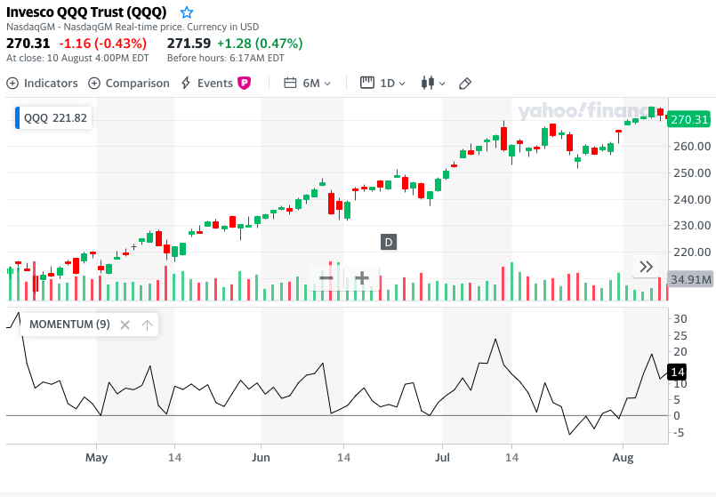
Here is an example of a stock chart with an indicator on a separate pane taken from Yahoo! Finance:

這是一個股票圖表的示例，該圖表在一個單獨的窗格中帶有從Yahoo!獲取的指標。 財務 ：

With this post, we want to explore how to create similar charts using Matplotlib. We also want to explore how to harness Matplotlib’s potential for customization and create original, publication-quality charts. To start with, we will learn how we can obtain that kind of subplot using Matplotlib. Then, we will apply that to plot our first technical indicator below the price, the Rate of Change (or ROC). We will then have a look at how to do that on an OHLC bar or Candlestick chart instead of a line chart.

在這篇文章中，我們想探討如何使用Matplotlib創建類似的圖表。 我們還想探索如何利用Matplotlib進行定制的潛力，并創建具有出版質量的原始圖表。 首先，我們將學習如何使用Matplotlib獲得這種子圖。 然后，我們將其應用到價格， 變化率 (或ROC )下繪制我們的第一個技術指標。 然后，我們將看看如何在OHLC條形圖或燭形圖而不是折線圖上執行此操作。

使用matplotlib的多個子圖 (Multiple subplots with matplotlib)

At this stage we need to delve into some technical aspects of how Matplotlib works: That is how we can harness its multiple plots capabilities and craft publishing quality charts. All the code provided assumes that you are using Jupyter Notebook. If instead, you are using a more conventional text editor or the command line, you will need to add:

在此階段，我們需要深入研究Matplotlib的工作原理的一些技術方面：這就是我們如何利用其多個繪圖功能并制作發布質量圖表的方式。 提供的所有代碼均假定您正在使用Jupyter Notebook 。 相反，如果您使用的是更常規的文本編輯器或命令行，則需要添加：

plt.show()

each time a chart is created in order to make it visible.

每次創建圖表以使其可見。

In the first two posts of this series we created our first financial price plots using the format:

在本系列的前兩篇文章中，我們使用以下格式創建了第一個金融價格圖：

plt.plot(dates, price, <additional parameters>)

You can see the first article on moving averages or the second on weighted and exponential moving averages.

您可以看到第一篇有關移動平均值的文章，或者第二篇有關加權和指數移動平均值的文章 。

When calling that method, matplotlib does a few things behind the scenes in order to create charts:

調用該方法時， matplotlib會在后臺執行一些操作以創建圖表：

• First, it creates an object called figure: this is the container where all of our charts are stored. A figure is created automatically and quietly, however, we can create it explicitly and access it when we need to pass some parameters, e.g. with the instruction: fig = plt.figure(figsize=(12,6))

  首先，它創建一個名為Figure的對象：這是存儲我們所有圖表的容器。 圖形是自動，安靜地創建的，但是，我們可以顯式創建它，并在需要傳遞某些參數時訪問它，例如，使用以下指令： fig = plt.figure(figsize=(12,6))

• On top of that, matplotlib creates an object called axes (do not confuse with axis): this object corresponds to a single subplot contained within the figure. Again, this action usually happens behind the scenes.

  最重要的是，matplotlib創建一個對象稱為軸 (不要混淆軸 )：該對象對應于一個單一副區包含圖之內。 同樣，此動作通常在幕后發生。

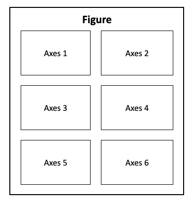
Within any figure, we can have multiple subplots (axes) arranged in a matrix:

在任何圖中 ，我們可以將多個子圖( 軸 )排列成一個矩陣：

我們的第一個多圖 (Our first multiple plot charts)

When it comes to charts with multiple subplots, there are enough ways and methods available to make our head spin. We are going to pick just one: the .subplot() method will serve our purposes well. Through other tutorials, you may come across a method called .add_subplot(): the .subplot() method is a wrapper for .add_subplots() (that means it should make its use simpler). With the exception of a few details, their use is actually very similar.

當涉及具有多個子圖的圖表時，有足夠的方法可以使我們旋轉。 我們將只選擇一種： .subplot()方法將很好地滿足我們的目的。 通過其他教程，你可能會遇到一個方法叫做.add_subplot()在.subplot()方法是一個包裝.add_subplots()這意味著它應該使它的使用更簡單)。 除了一些細節外，它們的用法實際上非常相似。

Whenever we add a subplot to a figure we need to supply three parameters:

每當我們向圖形添加子圖時，我們都需要提供三個參數：

• The number of rows in the chart matrix.
  圖表矩陣中的行數。
• The number of columns.
  列數。

• The number of the specific subplot: you can note from the diagram above that the axes objects are numbered going left to right, then top to bottom.

  特定子圖的編號：您可以從上圖中注意到， 軸對象的編號從左到右，然后從上到下。

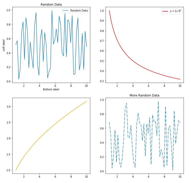
Let us try to build a practical example of a generic 2x2 multiple plot chart:

讓我們嘗試構建一個通用的2x2多重繪圖圖的實際示例：

Which gives us the following chart:

如下圖所示：

在價格序列中添加指標子圖 (Adding an indicator subplot to a price series)

Now that we know how to create charts with multiple plots, we can apply our skills to plot an indicator at the bottom of a price chart. For this task, we are going to use an indicator known as Rate of Change (ROC). There are actually a few different definitions of ROC, and the one that we are going to employ for our example is based on the formula:

既然我們知道如何創建包含多個圖表的圖表，我們就可以運用我們的技能在價格圖表的底部繪制一個指標。 對于此任務，我們將使用稱為變化率 ( ROC )的指標。 實際上，ROC有一些不同的定義，我們將在本示例中采用的定義基于以下公式：

where lag can be any whole number greater than zero and represents the number of periods (on a daily chart: days) we are looking back to compare our price. E.g., when we compute the ROC of the daily price with a 9-day lag, we are simply looking at how much, in percentage, the price has gone up (or down) compared to 9 days ago. In this article we are not going to discuss how to interpret the ROC chart and use it for investment decisions: that should better have a dedicated article and we are going to do that in a future post.

滯后可以是大于零的任何整數，并且代表周期數(在日線圖上為天)，我們正在回頭比較價格。 例如，當我們以9天的滯后時間計算每日價格的ROC時，我們只是在看價格與9天前相比上漲(或下跌)了多少(以百分比表示)。 在本文中，我們將不討論如何解釋ROC圖表并將其用于投資決策：最好有一篇專門的文章，我們將在以后的文章中進行介紹。

We start by preparing our environment:

我們從準備環境開始：

import pandas as pd
import numpy as np
import matplotlib.pyplot as plt# Required by pandas: registering  matplotlib date converters
pd.plotting.register_matplotlib_converters()# If you are using Jupyter, use this to show the output images within the Notebook:
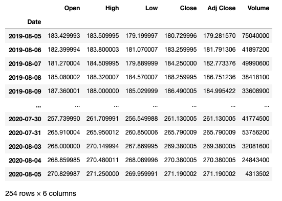
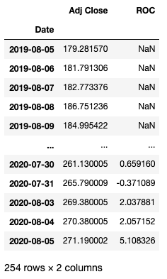
%matplotlib inline

For this exercise, I downloaded from Yahoo! Finance daily prices for the Invesco QQQ Trust, an ETF that tracks the performance of the Nasdaq 100 Index. You can find here the CSV file that I am using. We can load our data and have a glimpse at it:

對于本練習，我從Yahoo!下載。 跟蹤納斯達克100指數表現的ETF Invesco QQQ Trust的每日價格。 您可以在這里找到我正在使用的CSV文件 。 我們可以加載數據并瀏覽一下：

datafile = 'QQQ.csv'
data = pd.read_csv(datafile, index_col = 'Date')# Converting the dates from string to datetime format:
data.index = pd.to_datetime(data.index)data

Which looks like:

看起來像：

We can then compute a ROC series with a 9-day lag and add it as a column to our data frame:

然后，我們可以計算出滯后9天的ROC系列，并將其作為一列添加到我們的數據框中：

lag = 9
data['ROC'] = ( data['Adj Close'] / data['Adj Close'].shift(lag) -1 ) * 100data[['Adj Close', 'ROC']]

Which outputs:

哪個輸出：

To make our example charts easier to read, we use only a selection of our available data. Here is how we select the last 100 rows, corresponding to the 100 most recent trading days:

為了使示例圖表更易于閱讀，我們僅使用部分可用數據。 這是我們如何選擇最后100行(對應于最近100個交易日)的方式：

data_sel = data[-100:]
dates = data_sel.index
price = data_sel['Adj Close']
roc = data_sel['ROC']

We are now ready to create our first multiple plot chart, with the price at the top and the ROC indicator at the bottom. We can note that, compared to a generic chart with subplots, our indicator has the same date and time (the horizontal axis) as the price chart:

現在，我們準備創建我們的第一個多幅圖，價格在頂部，ROC指標在底部。 我們可以注意到，與帶有子圖的普通圖表相比，我們的指標具有與價格圖表相同的日期和時間(水平軸)：

fig = plt.figure(figsize=(12,10))# The price subplot:
price_ax = plt.subplot(2,1,1)
price_ax.plot(dates, price)# The ROC subplot shares the date axis with the price plot:
roc_ax = plt.subplot(2,1,2, sharex=price_ax)
roc_ax.plot(roc)# We can add titles to each of the subplots:
price_ax.set_title("QQQ  - Adjusted Closing Price")
roc_ax.set_title("9-Day ROC")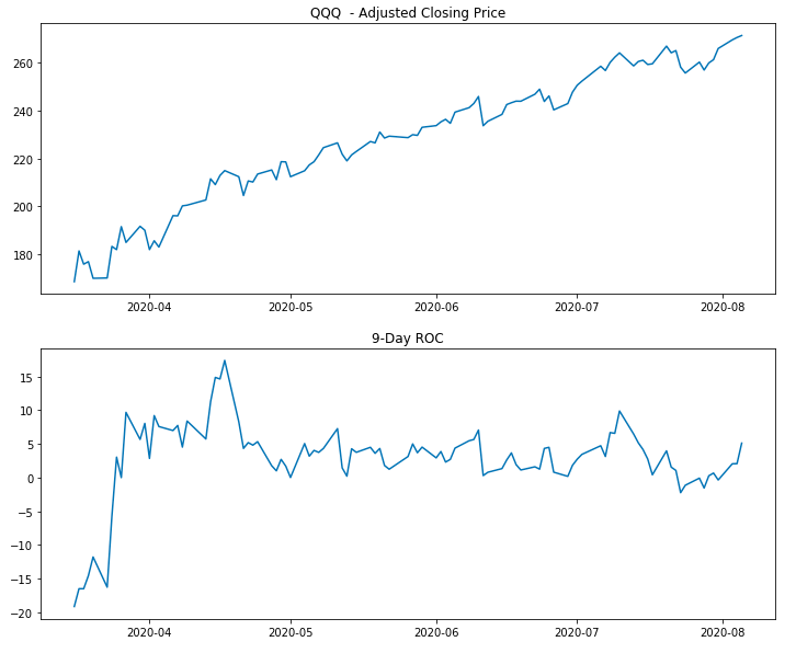

We have just plotted our first chart with price and ROC in separate areas: this chart does its job in the sense that it makes both price and indicator visible. It does not, however, do it in a very visually appealing way. To start with, price and ROC share the same time axis: there is no need to apply the date labels again on both charts. We can remove them from the top chart by using:

我們剛剛在不同區域繪制了第一張圖表，其中包含價格和ROC：此圖表在使價格和指標均可見的意義上發揮了作用。 但是，它并不是以非常吸引人的方式進行的。 首先，價格和ROC共享相同的時間軸：無需在兩個圖表上再次應用日期標簽 。 我們可以使用以下方法從頂部圖表中刪除它們：

price_ax.get_xaxis().set_visible(False)

We can also remove the gap between the two subplots with:

我們還可以使用以下方法消除兩個子圖之間的差距 ：

fig.subplots_adjust(hspace=0)

It is also a good idea to add a horizontal line at the zero level of the ROC to make it more readable, as well as to add labels to both vertical axes.

在ROC的零位添加一條水平線以使其更具可讀性，并且在兩個垂直軸上都添加標簽也是一個好主意。

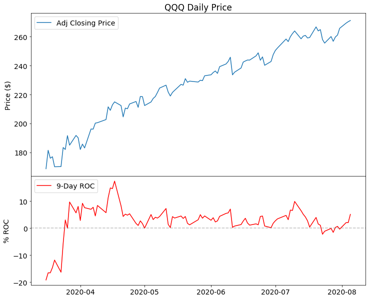
fig = plt.figure(figsize=(12,10))price_ax = plt.subplot(2,1,1)
price_ax.plot(dates, price, label="Adj Closing Price")
price_ax.legend(loc="upper left")roc_ax = plt.subplot(2,1,2, sharex=price_ax)
roc_ax.plot(roc, label="9-Day ROC", color="red")
roc_ax.legend(loc="upper left")price_ax.set_title("QQQ Daily Price")# Removing the date labels and ticks from the price subplot:
price_ax.get_xaxis().set_visible(False)# Removing the gap between the plots:
fig.subplots_adjust(hspace=0)# Adding a horizontal line at the zero level in the ROC subplot:
roc_ax.axhline(0, color = (.5, .5, .5), linestyle = '--', alpha = 0.5)# We can add labels to both vertical axis:
price_ax.set_ylabel("Price ($)")
roc_ax.set_ylabel("% ROC")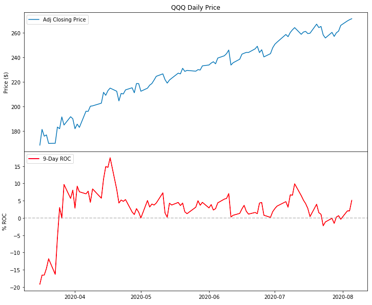

This chart looks already better. However, Matplotlib offers a much greater potential when it comes to creating professional-looking charts. Here are some examples of what we can do:

該圖表看起來已經更好。 但是，在創建具有專業外觀的圖表時，Matplotlib具有更大的潛力。 以下是一些我們可以做的例子：

• To enhance the readability of the ROC indicator, we can fill the areas between the plot and the horizontal line. The .fill_between() method will serve this purpose.

  為了提高ROC指標的可讀性，我們可以填充曲線圖和水平線之間的區域。 .fill_between()方法將用于此目的。

• We can format the date labels to show, for example, only the name of the month in short form (e.g., Jan, Feb, …).

  我們可以設置日期標簽的格式，以僅顯示簡短形式的月份名稱(例如Jan ， Feb …)。

• We can use a percent format for the labels on the ROC vertical axis.
  我們可以對ROC垂直軸上的標簽使用百分比格式。
• We can add a grid to both subplots and set a background color.
  我們可以將網格添加到兩個子圖中并設置背景顏色。
• Increase the margins (padding) between the plot and the borders.
  增加圖和邊框之間的邊距(邊距)。

• In order to maximize the chart’s Data-Ink Ratio, we can remove all the spines (the borders around the subplots) and the tick marks on the horizontal and vertical axis for both subplots.

  為了最大化圖表的數據墨水比 ，我們可以刪除兩個子圖的所有尖刺(子圖周圍的邊界)和水平和垂直軸上的刻度線。

• We can also set the default size for all the fonts to a larger number, say 14.
  我們還可以將所有字體的默認大小設置為更大的數字，例如14。

That is quite a long list of improvements. Without getting lost too much in the details, the following code should provide a good example:

這是一長串的改進。 不會在細節上迷失過多，以下代碼應提供一個很好的示例：

Which gives:

這使：

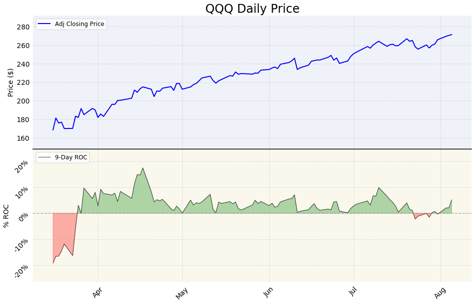
This chart provides a taster of what we can achieve by manipulating the default Matplotlib parameters. Of course, we can always achieve some visual improvements by applying an existing style sheet as we have done in the first article of this series, e.g. with:

該圖表提供了一個嘗試者，可以通過操作默認的Matplotlib參數來實現。 當然，我們總是可以通過應用現有樣式表來實現一些視覺上的改進，就像在本系列的第一篇文章中所做的那樣，例如：

plt.style.use('fivethirtyeight')

When using indicator subplots, most of the time we want the price section to take a larger area than the indicator section in the chart. To achieve this we need to manipulate the invisible grid that Matplotlib uses to place the subplots. We can do so using the GridSpec function. This is another very powerful feature of Matplotlib. I will just provide a brief example of how it can be used to control the height ratio between our two subplots:

當使用指標子圖時，大多數時候我們希望價格部分比圖表中的指標部分更大的面積。 為此，我們需要操縱Matplotlib用于放置子圖的不可見網格。 我們可以使用GridSpec 函數來實現 。 這是Matplotlib的另一個非常強大的功能。 我將提供一個簡短的示例，說明如何使用它來控制兩個子圖之間的高度比 ：

Which outputs:

哪個輸出：

As a side note, you may notice how this chart retained 14 as the font size set from the previous chart’s code. This happens because any changes to the rcParams Matplotlib parameters are permanent (until we restart the system). If we need to reset them we can use:

附帶說明一下，您可能會注意到此圖表如何保留14作為上一個圖表代碼中設置的字體大小。 發生這種情況是因為對rcParams Matplotlib參數的任何更改都是永久性的(直到重新啟動系統)。 如果我們需要重置它們，我們可以使用：

plt.style.use('default')

and add %matplotlib inline if we are using Jupyter Notebook.

如果我們使用的是Jupyter Notebook，則%matplotlib inline添加%matplotlib inline 。

OHLC和燭臺圖的指標 (Indicators with OHLC and Candlestick charts)

In all of the previous examples, we charted the price as a line plot. Line plots are a good way to visualize prices when we have only one data point (in this case, the closing price) for each period of trading. Quite often, with financial price series, we want to use OHLC bar charts or Candlestick charts: those charts can show all the prices that summarize the daily trading activity (Open, High, Low, Close) instead of just Close.

在所有前面的示例中，我們將價格繪制為線圖。 當我們在每個交易時段只有一個數據點(在本例中為收盤價)時，折線圖是可視化價格的好方法。 通常，對于金融價格系列，我們要使用OHLC條形圖或燭臺圖：這些圖可以顯示總結每日交易活動(開盤價，高價，低價，收盤價)的所有價格，而不僅僅是收盤價。

To plot OHLC bar charts and candlestick charts in Matplotlib we need to use the mplfinance library. As I mentioned in the previous post of this series, mplfinance development has gathered new momentum and things are rapidly evolving. Therefore, we will deal only cursorily on how to use it to create our charts.

要在Matplotlib中繪制OHLC條形圖和燭臺圖，我們需要使用mplfinance庫。 就像我在本系列的上 一篇 文章中提到的那樣 ， mplfinance的發展聚集了新的動力，并且事情正在Swift發展。 因此，我們將只粗略地討論如何使用它來創建圖表。

Mplfinance offers two methods to create subplots within charts and add an indicator:

Mplfinance提供了兩種在圖表內創建子圖并添加指標的方法：

• With the External Axes Method creating charts is more or less similar to what we have done so far. Mplfinance takes care of drawing the OHLC or candlesticks charts. We can then pass an Axes object with our indicator as a separate subplot.

  使用“ 外部軸方法”創建圖表與我們到目前為止所做的大致相似。 Mplfinance負責繪制OHLC或燭臺圖表。 然后，我們可以將帶有指標的軸對象作為單獨的子圖傳遞。

• The Panels Method is even easier to use than pure Matplotlib code: mplfinance takes control of all the plotting and styling operations for us. To manipulate the visual aspects of the chart we can apply existing styles or create our own style.

  面板方法甚至比純Matplotlib代碼更易于使用： mplfinance為我們控制了所有繪圖和樣式操作。 要操縱圖表的視覺效果，我們可以應用現有樣式或創建自己的樣式。

The External Axes Method was released less than a week ago from the time I am writing this. I am still looking forward to making use of it to find out what potential it can offer.

自撰寫本文之日起，不到一周前發布了“ 外部軸方法” 。 我仍然期待著利用它來發現它可以提供什么潛力。

As a taster of what we can do using the mplfinance Panel Method, we can plot a candlestick chart with the volume in a separate pane:

作為品嘗我們使用mplfinance面板方法可以做些什么的嘗試，我們可以在單獨的窗格中繪制燭臺圖和其體積：

import mplfinance as mpfmpf.plot(data_sel, type='candle',  style='yahoo', title="QQQ Daily Price", volume=True)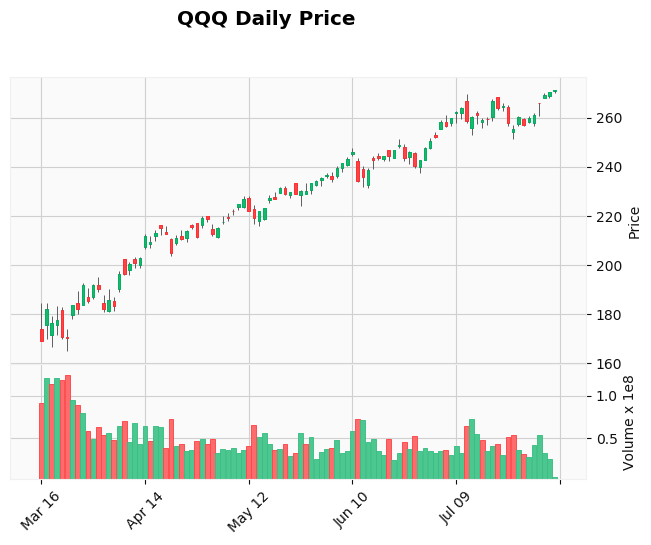

We can add our ROC indicator in a separate subplot too:

我們也可以在單獨的子圖中添加ROC指標：

# We create an additional plot placing it on the third panel
roc_plot = mpf.make_addplot(roc, panel=2, ylabel='ROC')#We pass the additional plot using the addplot parameter
mpf.plot(data_sel, type='candle',  style='yahoo', addplot=roc_plot, title="QQQ Daily Price", volume=True)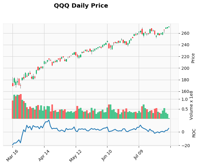

結論 (Conclusion)

There are several packages out there that make it possible to create financial charts using Python and pandas. In particular, plotly stands out for its capability to create good looking interactive charts. Matplotlib, on the other hand, may not produce the best charts straight out of the box (look at seaborn if you need that) however, it has a huge customization potential that makes it possible to create static charts that can stand out in a professional publication.

有幾種軟件包可以使用Python和pandas創建財務圖表。 特別是， plotly以其創建美觀的交互式圖表的能力而脫穎而出。 另一方面，Matplotlib可能無法立即生成最佳圖表(如果需要，請查看seaborn )，但是它具有巨大的自定義潛力，這使得創建靜態圖表可以在專業人士中脫穎而出。出版物。

That is why I believe it is well worth to get the grips on tweaking the properties of matplotlib. The future developments of mplfinance will make those possibilities even more appealing.

這就是為什么我認為調整一下matplotlib的屬性非常值得。 mplfinance的未來發展將使這些可能性更具吸引力。