數據eda
This banking data was retrieved from Kaggle and there will be a breakdown on how the dataset will be handled from EDA (Exploratory Data Analysis) to Machine Learning algorithms.
該銀行數據是從Kaggle檢索的,將詳細介紹如何將數據集從EDA(探索性數據分析)轉換為機器學習算法。
腳步: (Steps:)
- Identification of variables and data types 識別變量和數據類型
- Analyzing the basic metrics 分析基本指標
- Non-Graphical Univariate Analysis 非圖形單變量分析
- Graphical Univariate Analysis 圖形單變量分析
- Bivariate Analysis 雙變量分析
- Correlation Analysis 相關分析
資料集: (Dataset:)
The dataset that will be used is from Kaggle. The dataset is a bank loan dataset, making the goal to be able to detect if someone will fully pay or charge off their loan.
將使用的數據集來自Kaggle 。 該數據集是銀行貸款數據集,其目標是能夠檢測某人是否將完全償還或償還其貸款。
The dataset consist of 100,000 rows and 19 columns. The predictor (dependent variable) will be “Loan Status,” and the features (independent variables) will be the remaining columns.
數據集包含100,000行和19列。 預測變量(因變量)將為“貸款狀態”,要素(因變量)將為剩余的列。
變量識別: (Variable Identification:)
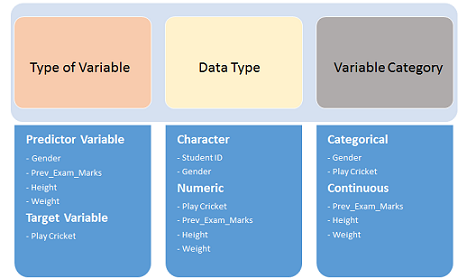
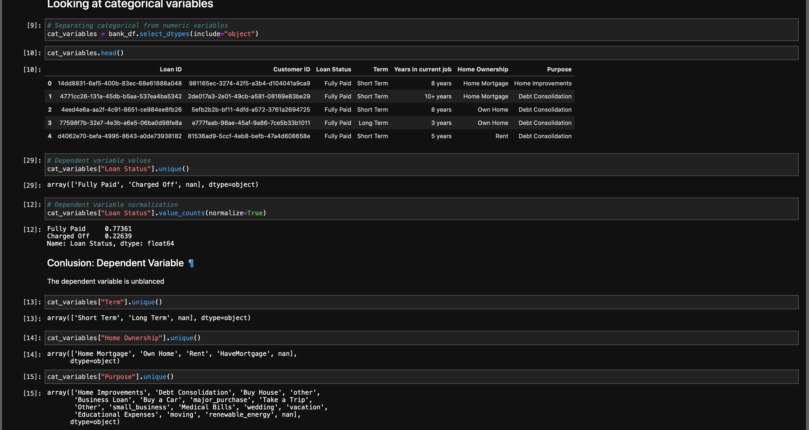
The very first step is to determine what type of variables we’re dealing with in the dataset.
第一步是確定數據集中要處理的變量類型。
df.head()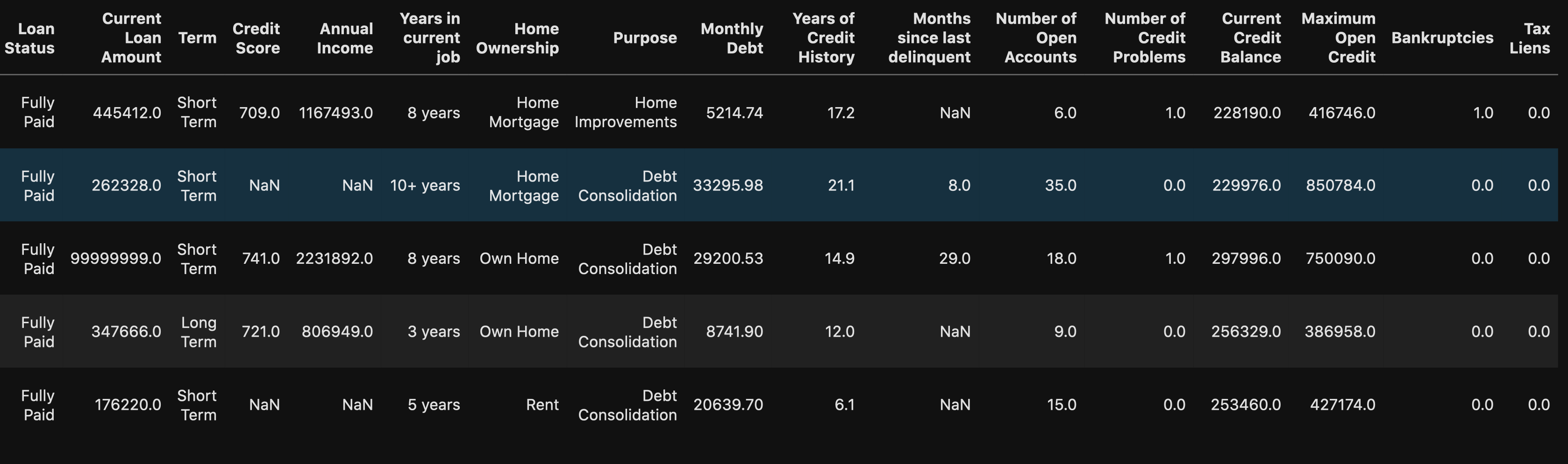
We can see that there are some numeric and string (object) data types in our dataset. But to be certain, you can use:
我們可以看到我們的數據集中有一些數字和字符串(對象)數據類型。 但可以肯定的是,您可以使用:
df.info() # Shows data types for each column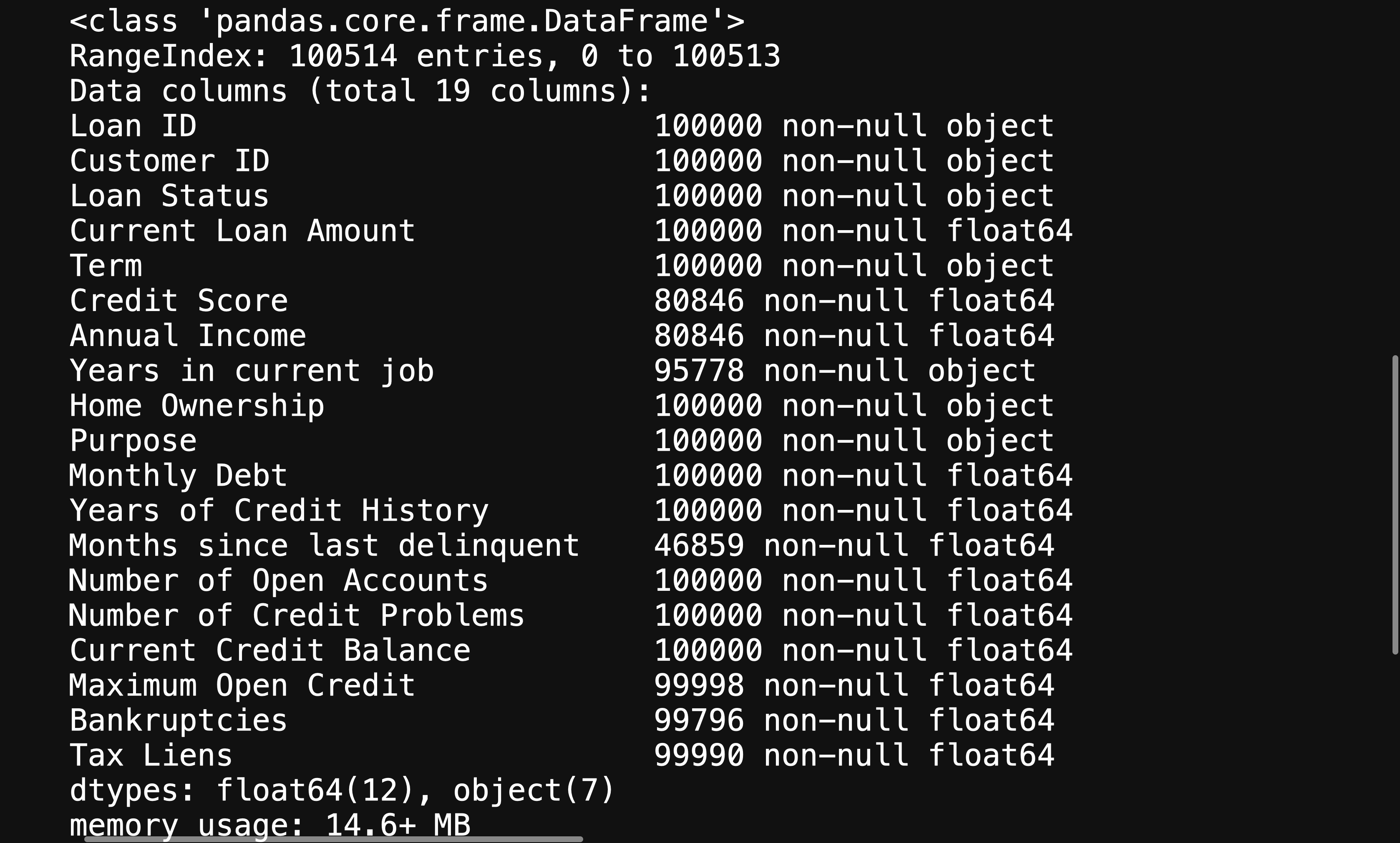
This will give you further information about your variables, helping you figure out what will need to be changed in order to help your machine learning algorithm be able to interpret your data.
這將為您提供有關變量的更多信息,幫助您確定需要更改哪些內容,以幫助您的機器學習算法能夠解釋您的數據。
分析基本指標 (Analyzing Basic Metrics)
This will be as simple as using:
這就像使用以下命令一樣簡單:
df.describe().T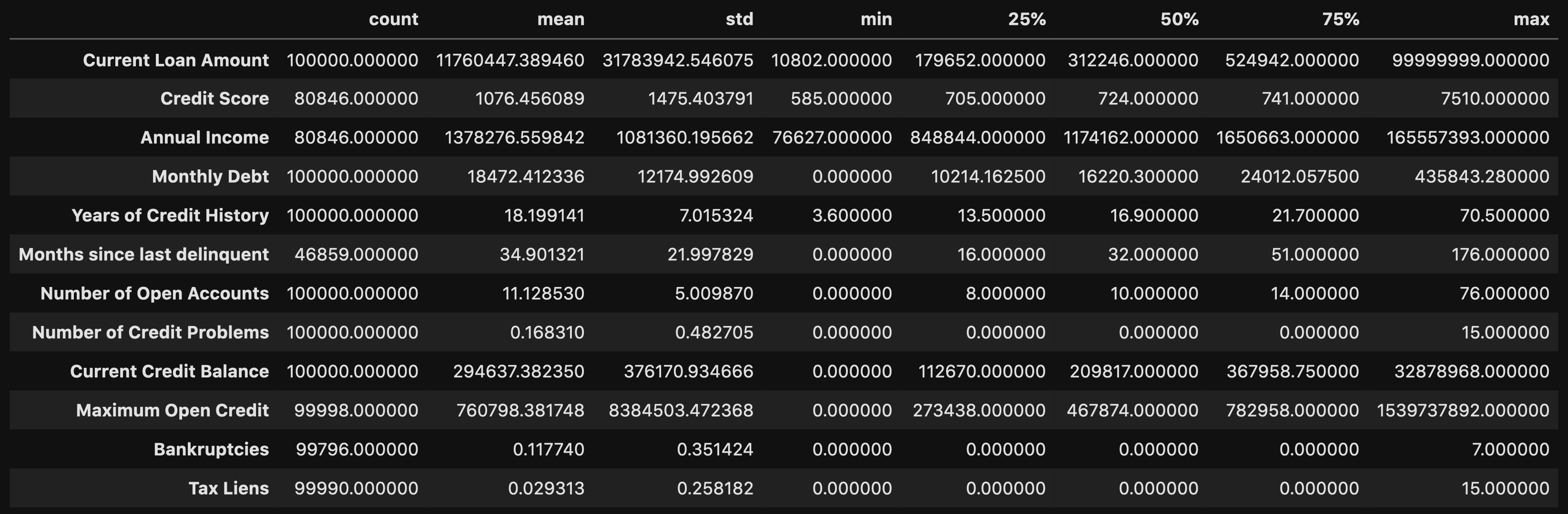
This allows you to look at certain metrics, such as:
這使您可以查看某些指標,例如:
- Count — Amount of values in that column 計數-該列中的值數量
- Mean — Avg. value in that column 均值-平均 該列中的值
- STD(Standard Deviation) — How spread out your values are STD(標準偏差)—您的價值觀分布如何
- Min — The lowest value in that column 最小值-該列中的最小值
- 25% 50% 70%— Percentile 25%50%70%—百分位數
- Max — The highest value in that column 最大值-該列中的最大值
From here you can identify what your values look like, and you can detect if there are any outliers.
在這里,您可以確定值的外觀,并可以檢測是否存在異常值。
From doing the .describe() method, you can see that there are some concerning outliers in Current Loan Amount, Credit Score, Annual Income, and Maximum Open Credit.
通過執行.describe()方法,您可以看到在當前貸款額,信用評分,年收入和最大未結信貸中存在一些與異常有關的問題。
非圖形單變量分析 (Non-Graphical Univariate Analysis)
Univariate Analysis is when you look at statistical data in your columns.
單變量分析是當您查看列中的統計數據時。
This can be as simple as doing df[column].unique() or df[column].value_counts(). You’re trying to get as much information from your variables as possible.
這可以像執行df [column] .unique()或df [column] .value_counts()一樣簡單。 您正在嘗試從變量中獲取盡可能多的信息。
You also want to find your null values
您還想找到空值
df.isna().sum()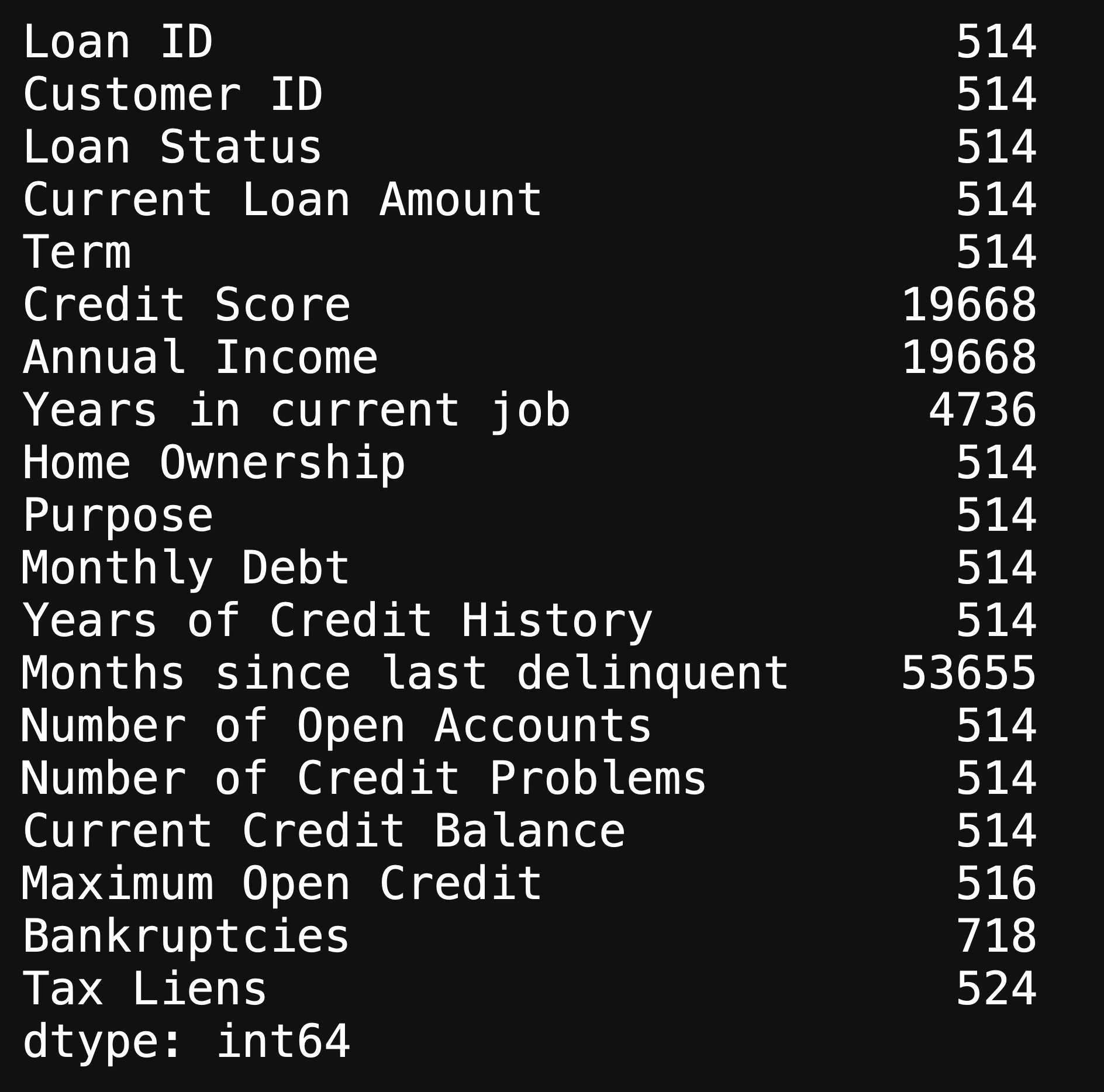
This will show you the amount of null values in each column, and there are an immense amount of missing values in our dataset. We will look further into the missing values when doing Graphical Univariate Analysis.
這將向您顯示每列中的空值數量,并且我們的數據集中有大量的缺失值。 在進行圖形單變量分析時,我們將進一步研究缺失值。
圖形單變量分析 (Graphical Univariate Analysis)
Here is when we look at our variables using graphs.
這是我們使用圖形查看變量的時候。
We can use a bar plot in order to look at our missing values:
我們可以使用條形圖來查看缺失值:
fig, ax = plt.subplots(figsize=(15, 5))x = df.isna().sum().index
y = df.isna().sum()
ax.bar(x=x, height=y)
ax.set_xticklabels(x, rotation = 45)
plt.tight_layout();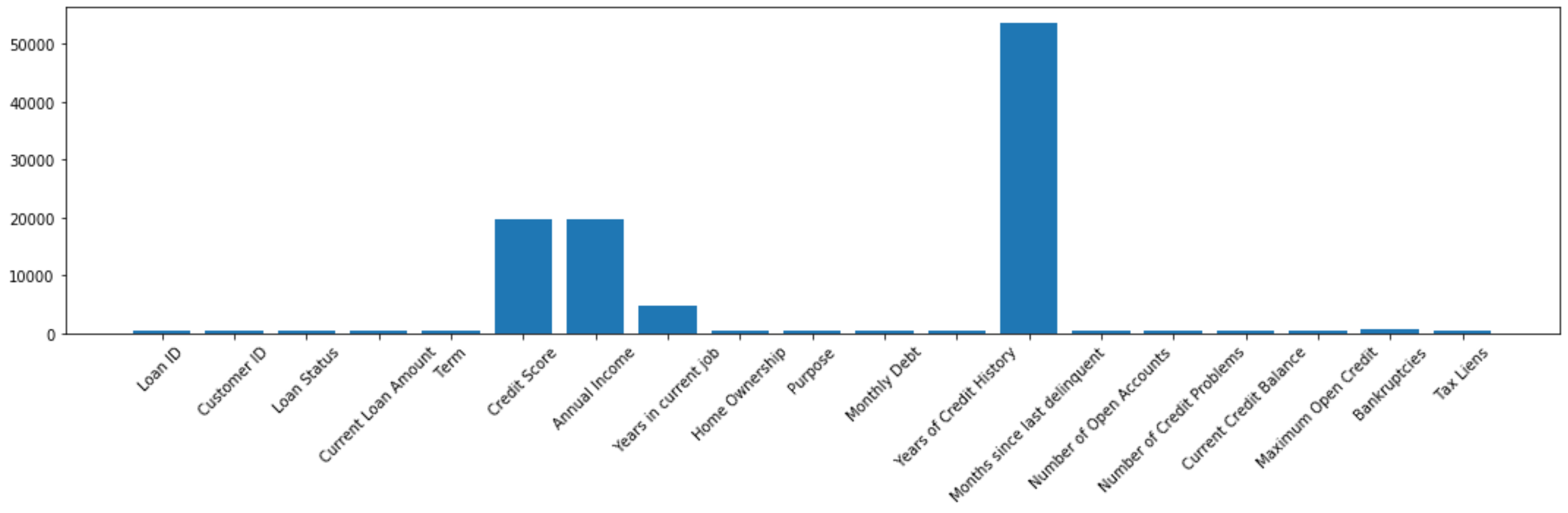
Moving past missing values, we can also use histograms to look at the distribution of our features.
超越缺失值后,我們還可以使用直方圖查看特征的分布。
df["Years of Credit History"].hist(bins=200)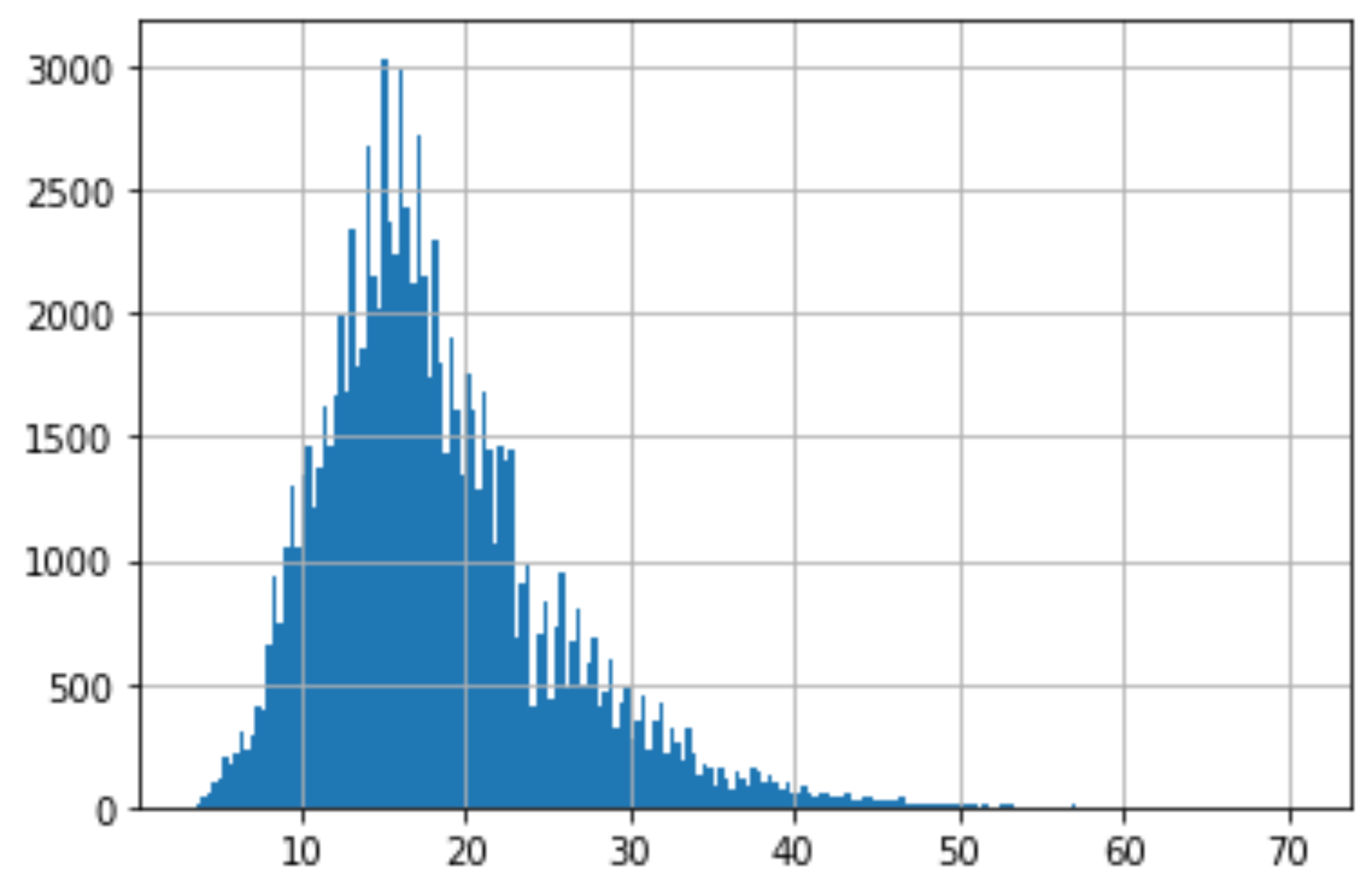
From this histogram you are able to detect if there are any outliers by seeing if it is left or right skew, and the one that we are looking at is a slight right skew.
從此直方圖中,您可以通過查看它是否是左偏斜或右偏斜來檢測是否存在異常值,而我們正在查看的是一個稍微偏斜的偏斜。
We ideally want our histograms for each feature to be close to a normal distribution as possible.
理想情況下,我們希望每個功能的直方圖盡可能接近正態分布。
# Checking credit score
df["Credit Score"].hist(bins=30)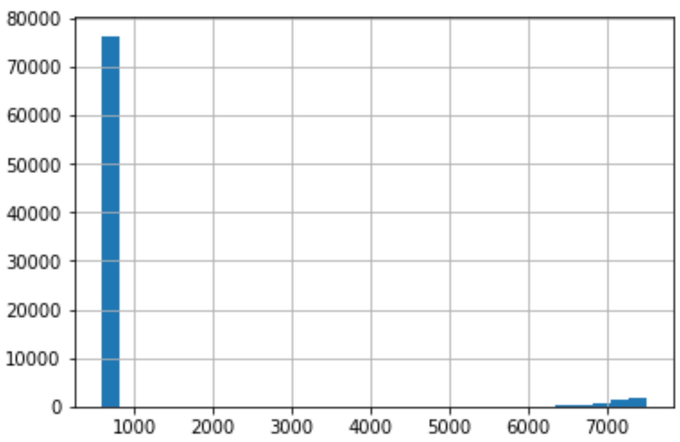
As we do the same thing for Credit Score, we can see that there is an immense right skew that rest in the thousands. This is very concerning because for our dataset, Credit Score is supposed to be at a 850 cap.
當我們對信用評分執行相同的操作時,我們可以看到存在成千上萬的巨大右偏。 這非常令人擔憂,因為對于我們的數據集而言,信用評分應設置為850上限。
Lets take a closer look:
讓我們仔細看看:
# Rows with a credit score greater than 850, U.S. highest credit score.
df.loc[df["Credit Score"] > 850]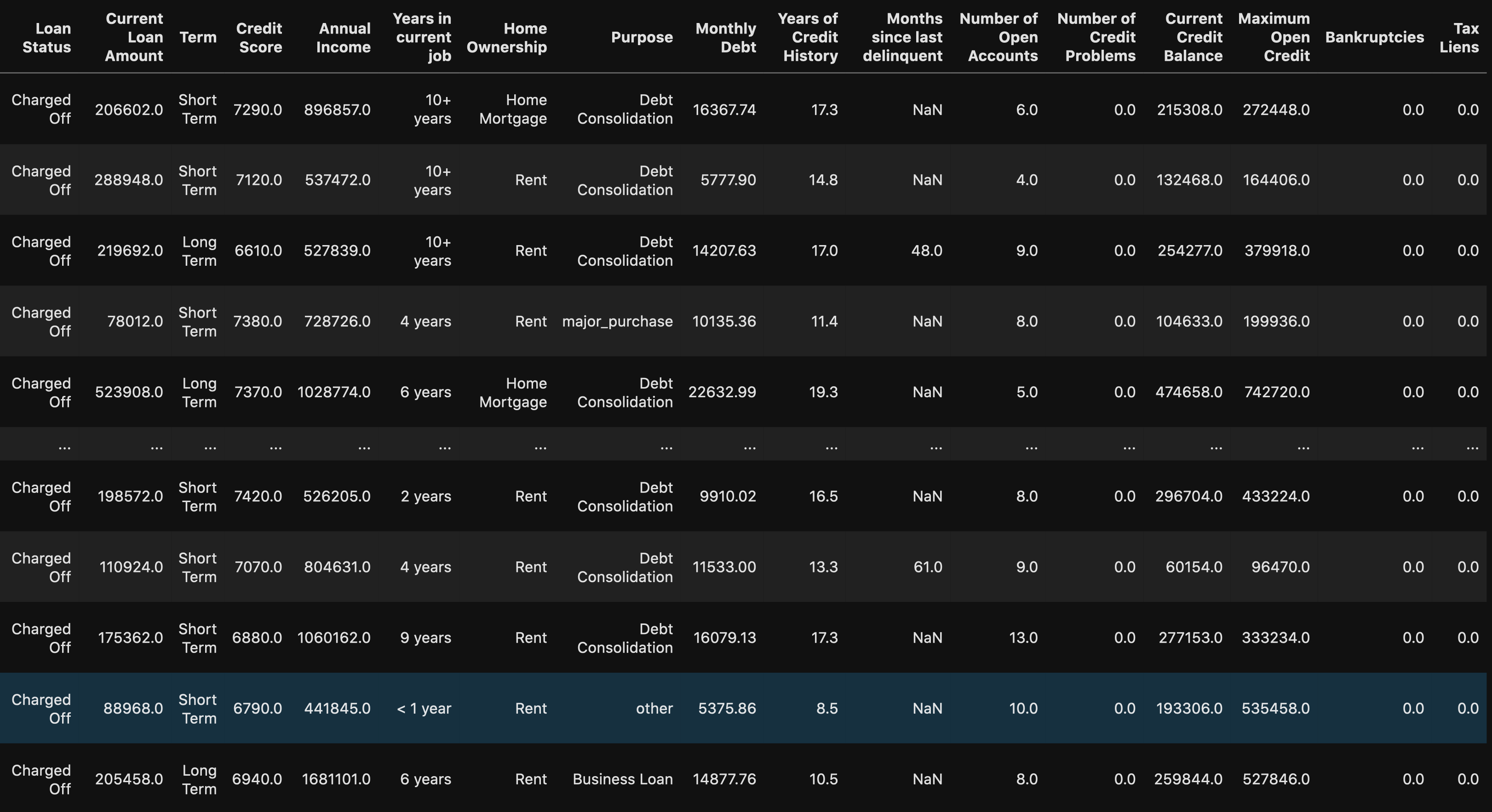
When using the loc method you are able to see all of the rows with a credit score greater than 850. We can see that this might be a human error because there are 0’s added on to the end of the values. This will be an easy fix once we get to processing the data.
使用loc方法時,您可以看到所有信用評分大于850的行。我們可以看到這可能是人為錯誤,因為在值的末尾添加了0。 一旦我們開始處理數據,這將是一個簡單的修復。
Another way to detect outliers are to use box plots and scatter plots.
檢測離群值的另一種方法是使用箱形圖和散點圖。
fig, ax = plt.subplots(4, 3)# Setting height and width of subplots
fig.set_figheight(15)
fig.set_figwidth(30)# Adding spacing between boxes
fig.tight_layout(h_pad=True, w_pad=True)sns.boxplot(bank_df["Number of Open Accounts"], ax=ax[0, 0])
sns.boxplot(bank_df["Current Loan Amount"], ax=ax[0, 1])
sns.boxplot(bank_df["Monthly Debt"], ax=ax[0, 2])
sns.boxplot(bank_df["Years of Credit History"], ax=ax[1, 0])
sns.boxplot(bank_df["Months since last delinquent"], ax=ax[1, 1])
sns.boxplot(bank_df["Number of Credit Problems"], ax=ax[1, 2])
sns.boxplot(bank_df["Current Credit Balance"], ax=ax[2, 0])
sns.boxplot(bank_df["Maximum Open Credit"], ax=ax[2, 1])
sns.boxplot(bank_df["Bankruptcies"], ax=ax[2, 2])
sns.boxplot(bank_df["Tax Liens"], ax=ax[3, 0])plt.show()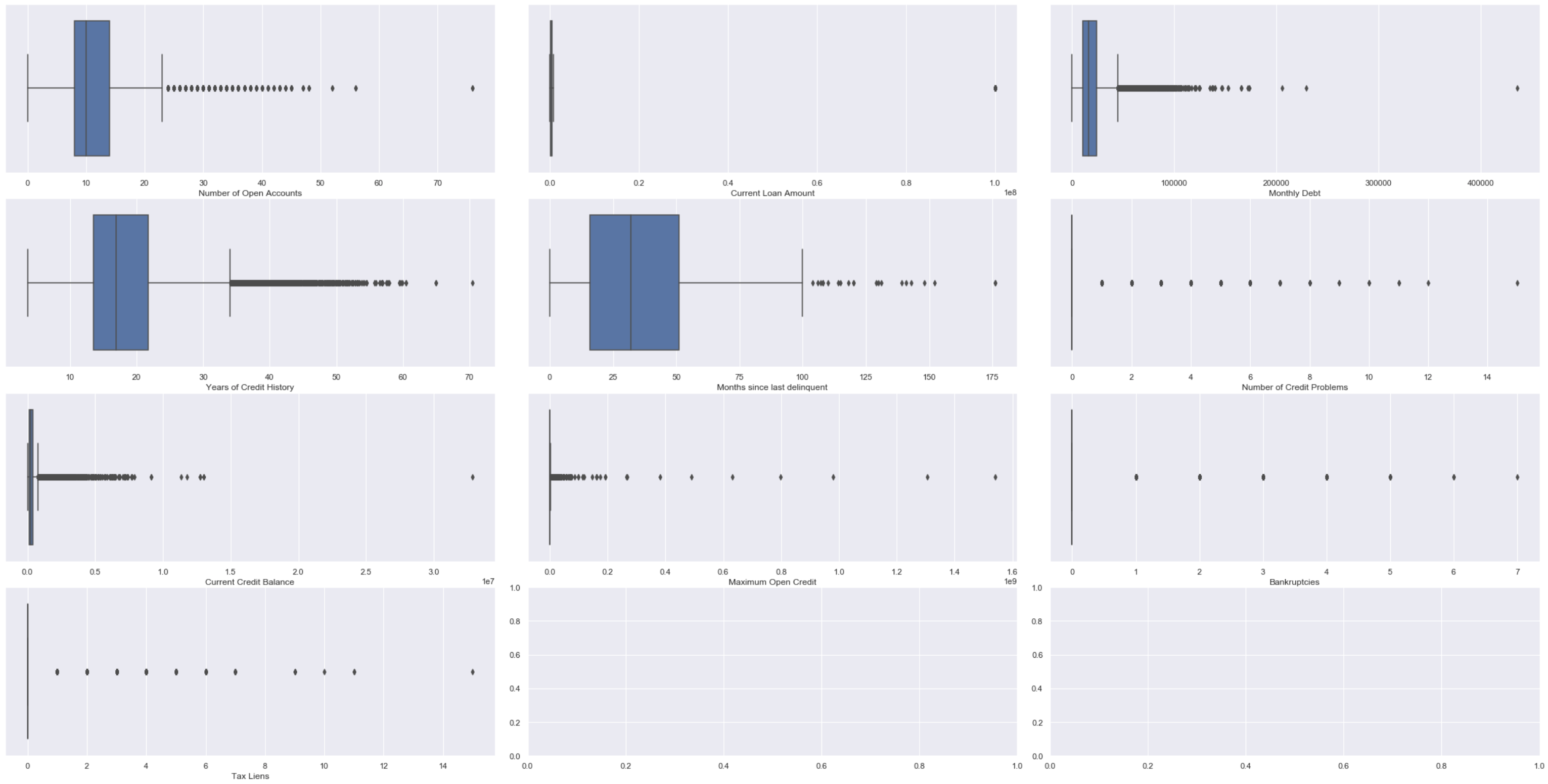
fig, ax = plt.subplots(4, 3)# Setting height and width of subplots
fig.set_figheight(15)
fig.set_figwidth(30)# Adding spacing between boxes
fig.tight_layout(h_pad=True, w_pad=True)sns.scatterplot(data=bank_df["Number of Open Accounts"], ax=ax[0, 0])
sns.scatterplot(data=bank_df["Current Loan Amount"], ax=ax[0, 1])
sns.scatterplot(data=bank_df["Monthly Debt"], ax=ax[0, 2])
sns.scatterplot(data=bank_df["Years of Credit History"], ax=ax[1, 0])
sns.scatterplot(data=bank_df["Months since last delinquent"], ax=ax[1, 1])
sns.scatterplot(data=bank_df["Number of Credit Problems"], ax=ax[1, 2])
sns.scatterplot(data=bank_df["Current Credit Balance"], ax=ax[2, 0])
sns.scatterplot(data=bank_df["Maximum Open Credit"], ax=ax[2, 1])
sns.scatterplot(data=bank_df["Bankruptcies"], ax=ax[2, 2])
sns.scatterplot(data=bank_df["Tax Liens"], ax=ax[3, 0])plt.show()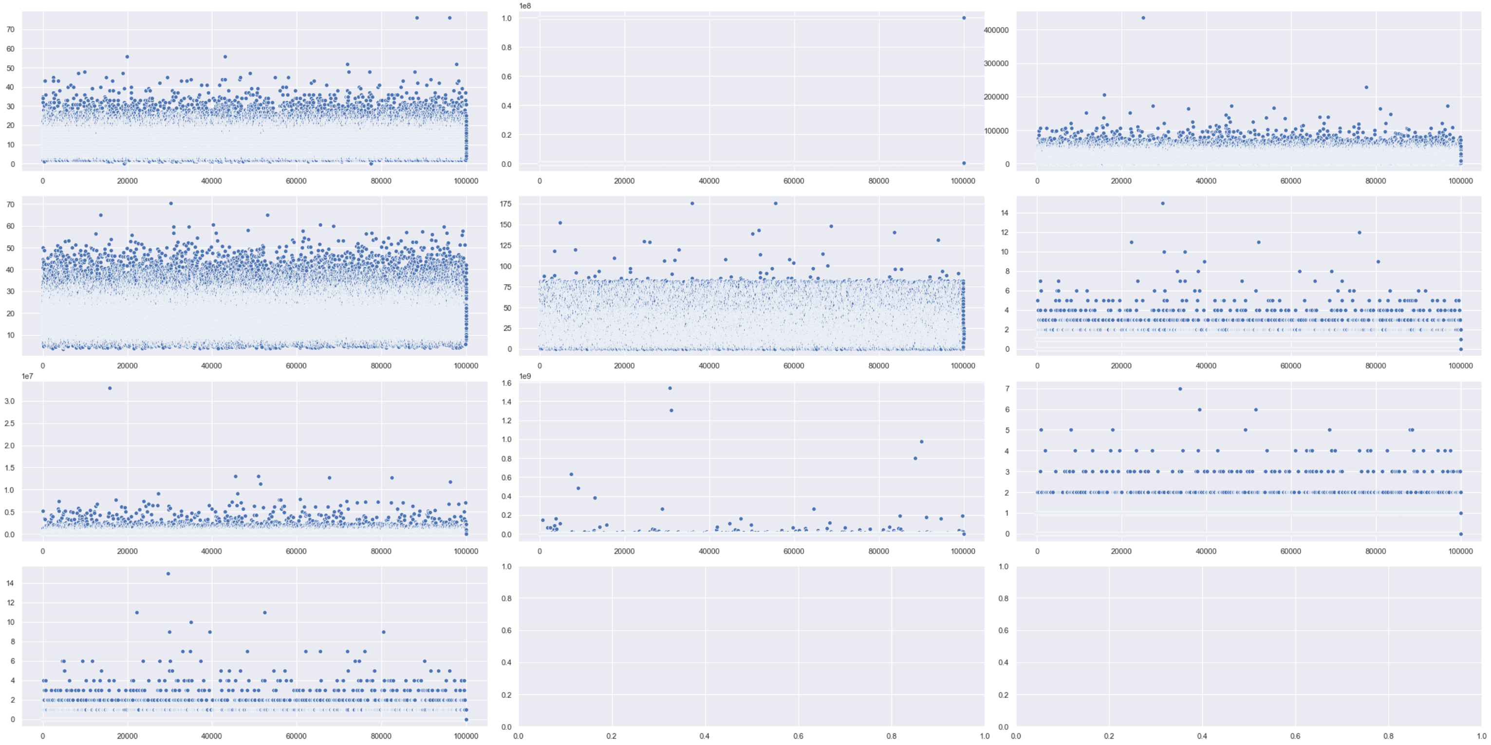
相關分析 (Correlation Analysis)
Correlation is when you want to detect how one variable reacts to another. What you don’t want is multicollinearity and to check for that you can use:
關聯是當您要檢測一個變量對另一個變量的React時。 您不想要的是多重共線性,并且可以使用以下方法進行檢查:
# Looking at mulitcollinearity
sns.heatmap(df.corr())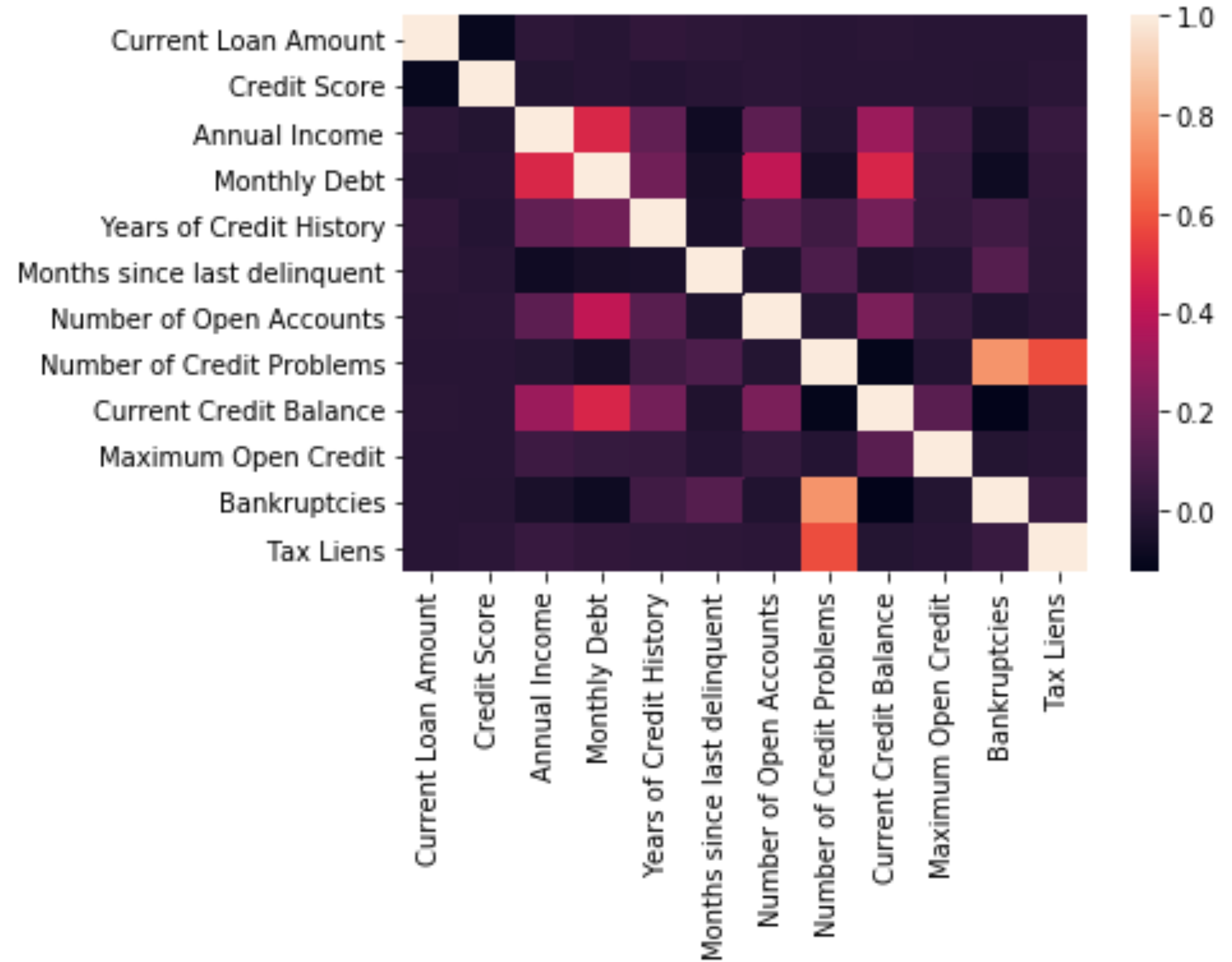
翻譯自: https://medium.com/analytics-vidhya/bank-data-eda-step-by-step-67a61a7f1122
數據eda
本文來自互聯網用戶投稿,該文觀點僅代表作者本人,不代表本站立場。本站僅提供信息存儲空間服務,不擁有所有權,不承擔相關法律責任。 如若轉載,請注明出處:http://www.pswp.cn/news/391690.shtml 繁體地址,請注明出處:http://hk.pswp.cn/news/391690.shtml 英文地址,請注明出處:http://en.pswp.cn/news/391690.shtml
如若內容造成侵權/違法違規/事實不符,請聯系多彩編程網進行投訴反饋email:809451989@qq.com,一經查實,立即刪除!相關文章


計算機網絡原理筆記-三次握手
)
VB2010 的隱式續行(Implicit Line Continuation)

flutter bloc_如何在Flutter中使用Streams,BLoC和SQLite

leetcode 303. 區域和檢索 - 數組不可變

Bigmart數據集銷售預測

Android控制ScrollView滑動速度

數據特征分析-帕累托分析
)
leetcode 304. 二維區域和檢索 - 矩陣不可變(前綴和)

算法訓練營 重編碼_編碼訓練營后如何找到工作

dt決策樹_決策樹:構建DT的分步方法

讀C#開發實戰1200例子記錄-2017年8月14日10:03:55
閃退異常上報撲獲日志集成與使用指南)
iOS端(騰訊Bugly)閃退異常上報撲獲日志集成與使用指南

數據特征分析-正太分布

leetcode 338. 比特位計數

r語言調用數據集中的數據集_自然語言數據集中未解決的問題
功能分支)
為什么不應該使用(長期存在的)功能分支
 Spring 3 報org.aopalliance.intercept.MethodInterceptor問題解決方法)
(轉) Spring 3 報org.aopalliance.intercept.MethodInterceptor問題解決方法

數據特征分析-相關性分析
)