Note: This post is heavy on code, but yes well documented.

注意：這篇文章講的是代碼，但確實有據可查。

問題描述 (The Problem Description)

The data scientists at BigMart have collected 2013 sales data for 1559 products across 10 stores in different cities. Also, certain attributes of each product and store have been defined. The aim is to build a predictive model and find out the sales of each product at a particular store.

BigMart的數據科學家收集了2013年不同城市10家商店中1559種產品的銷售數據。 另外，已經定義了每個產品和商店的某些屬性。 目的是建立預測模型并找出特定商店中每種產品的銷售情況。

Using this model, BigMart will try to understand the properties of products and stores which play a key role in increasing sales.

BigMart將使用此模型嘗試了解在增加銷售額中起關鍵作用的產品和商店的屬性。

Find the entire notebook on GitHub: BigMart Sales Prediction

在GitHub上找到整個筆記本： BigMart銷售預測

Metric Used — Root Mean Squared Error

使用的度量 標準—均方根誤差

I achieved an RMSE of 946.34. Thanks to K-Fold Cross Validation, Random Forest Regressor and obviously enough patience.

我的RMSE為946.34。 多虧了K折交叉驗證，Random Forest Regressor和明顯的耐心。

You can find the dataset here: DATASET

您可以在此處找到數據集： DATASET

First lets get a feel of the data

首先讓我們感受一下數據

train.dtypesItem_Identifier               object
Item_Weight                  float64
Item_Fat_Content              object
Item_Visibility              float64
Item_Type                     object
Item_MRP                     float64
Outlet_Identifier             object
Outlet_Establishment_Year      int64
Outlet_Size                   object
Outlet_Location_Type          object
Outlet_Type                   object
Item_Outlet_Sales            float64
dtype: object

檢查表是否缺少值 (Checking if table has missing values)

train.isnull().sum(axis=0)Item_Identifier                 0
Item_Weight                  1463
Item_Fat_Content                0
Item_Visibility                 0
Item_Type                       0
Item_MRP                        0
Outlet_Identifier               0
Outlet_Establishment_Year       0
Outlet_Size                  2410
Outlet_Location_Type            0
Outlet_Type                     0
Item_Outlet_Sales               0
dtype: int64

Item_Weight has 1463 and Outlet_Size has 2410 missing values

Item_Weight有1463，Outlet_Size有2410缺失值

train.describe()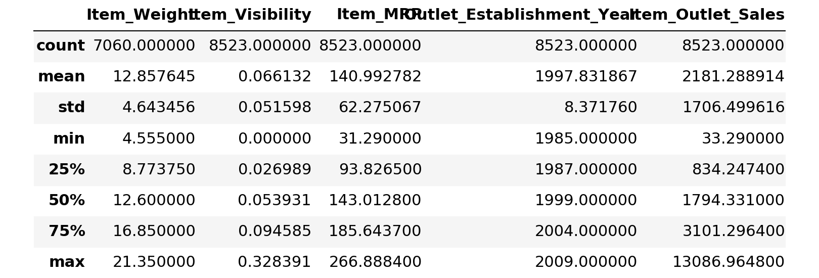

讓我們做一些數據可視化！ (Lets do some Data Viz!)

Hmm.. Items having visibility less than 0.2 sold them most

可見度小于0.2的商品最多

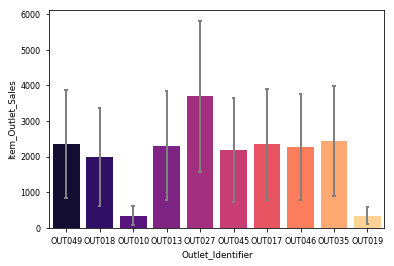
.Top 2 Contributors: Outlet_27 > Outlet_35
.Bottom 2 Contributors: Outlet 10 & Outlet 19

讓我們檢查一下哪種物品類型的銷量最高 (Lets check which item type sold the most)

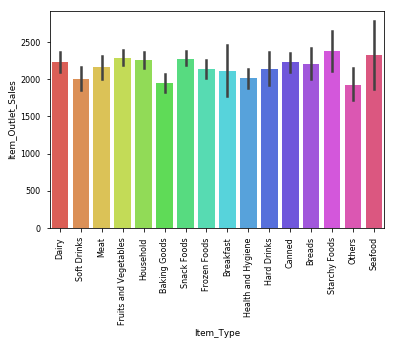
檢查異常值 (Checking for outliers)

.Health and hygiene has an outlier

這里是有趣的部分！ (Here comes the FUN part!!)

資料清理 (DATA CLEANING)

Peeking into what kind of values Item_Fat_Content and Item_Visibility contains.

窺視Item_Fat_Content和Item_Visibility包含哪些類型的值。

train.Item_Fat_Content.value_counts() # has mismatched factor levelsLow Fat    5089
Regular    2889
LF          316
reg         117
low fat     112
Name: Item_Fat_Content, dtype: int64train.Item_Visibility.value_counts().head()0.000000    526
0.076975      3
0.041283      2
0.085622      2
0.187841      2
Name: Item_Visibility, dtype: int64

Strange!! Item Visibility cant be 0. Lets keep a note of that for now.

奇怪！！ 項目可見性不能為0。暫時保留一下。

train.Outlet_Size.value_counts()Medium    2793
Small     2388
High       932
Name: Outlet_Size, dtype: int64

到目前為止，從數據集中的快速觀察： (Quick observations from the dataset so far:)

1.Item_Fat_Content has mismatched factor levels
2.Min(Item_visibility) = 0. Not practically possible. Treat 0's as missing values
3.Item_weight has 1463 missing values
4.Outlet_Size has unmatched factor levels

數據插補 (Data Imputation)

Filling outlet size

灌裝口尺寸

My opinion: Outlet size depends on outlet type and the location of the outlet

我的看法：插座尺寸取決于插座類型和插座位置

crosstable = pd.crosstab(train['Outlet_Size'],train['Outlet_Type'])
crosstable

This is why I love the crosstab feature ?

這就是為什么我喜歡交叉表功能?

From the above table it is evident that all the grocery stores are of small types, which is mostly true in the real world.

從上表可以看出，所有雜貨店都是小型的，這在現實世界中大多是正確的。

Therefore mapping Grocery store and small size

因此，映射雜貨店和小尺寸

dic = {'Grocery Store':'Small'}
s = train.Outlet_Type.map(dic)train.Outlet_Size= train.Outlet_Size.combine_first(s)
train.Outlet_Size.value_counts()Small     2943
Medium    2793
High       932
Name: Outlet_Size, dtype: int64# Checking if imputation was successful
train.isnull().sum(axis=0)Item_Identifier                 0
Item_Weight                  1463
Item_Fat_Content                0
Item_Visibility                 0
Item_Type                       0
Item_MRP                        0
Outlet_Identifier               0
Outlet_Establishment_Year       0
Outlet_Size                  1855
Outlet_Location_Type            0
Outlet_Type                     0
Item_Outlet_Sales               0
dtype: int64

In real world it is mostly seen that outlet size varies with the location of the outlet, hence checking between the same

在現實世界中，大多數情況下會看到插座的尺寸隨插座的位置而變化，因此在相同插座之間進行檢查

From the above table it is evident that all the Tier 2 stores are of small types. Therefore mapping Tier 2 store and small size

從上表可以看出，所有第2層商店都是小型商店。 因此，映射第2層商店且尺寸較小

dic = {"Tier 2":"Small"}
s = train.Outlet_Location_Type.map(dic)
train.Outlet_Size = train.Outlet_Size.combine_first(s)train.isnull().sum(axis=0)Item_Identifier                 0
Item_Weight                  1463
Item_Fat_Content                0
Item_Visibility                 0
Item_Type                       0
Item_MRP                        0
Outlet_Identifier               0
Outlet_Establishment_Year       0
Outlet_Size                     0
Outlet_Location_Type            0
Outlet_Type                     0
Item_Outlet_Sales               0
dtype: int64train.Item_Identifier.value_counts().sum()8523

Outlet size missing values have been imputed

出口尺寸缺失值已估算

Imputing for Item_Weight

估算Item_Weight

Instead of imputing with the overall mean of all the items. It would be better to impute it with the mean of particular item type — Food,Drinks,Non-Consumable. Did this as some products may be on the heavier side and some on the lighter.

而不是用所有項目的整體平均值來估算。 最好用特定項目類型的平均值(食物，飲料，非消耗品)來估算。 這樣做是因為某些產品可能偏重而某些產品較輕。

#Fill missing values of weight of Item According to means of Item Identifier
train['Item_Weight']=train['Item_Weight'].fillna(train.groupby('Item_Identifier')['Item_Weight'].transform('mean'))train.isnull().sum()Item_Identifier              0
Item_Weight                  4
Item_Fat_Content             0
Item_Visibility              0
Item_Type                    0
Item_MRP                     0
Outlet_Identifier            0
Outlet_Establishment_Year    0
Outlet_Size                  0
Outlet_Location_Type         0
Outlet_Type                  0
Item_Outlet_Sales            0
dtype: int64train[train.Item_Weight.isnull()]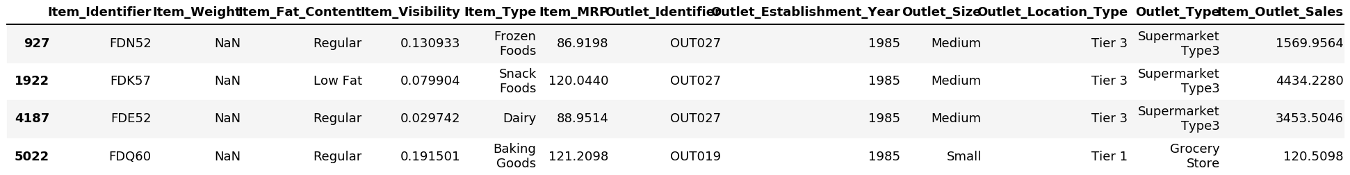

The above 4 item weights weren’t imputed because in the dataset there is only one record for each of them. Hence mean could not be calculated.

上面的4個項目權重沒有被估算，因為在數據集中每個項只有一條記錄。 因此，均值無法計算。

So, we will fill Item_Weight by the corresponding Item_Type for these 4 values

因此，我們將使用這4個值的相應Item_Type填充Item_Weight

# List of item types item_type_list = train.Item_Type.unique().tolist()# grouping based on item type and calculating mean of item weightItem_Type_Means = train.groupby('Item_Type')['Item_Weight'].mean()# Mapiing Item weight to item type meanfor i in item_type_list:
    dic = {i:Item_Type_Means[i]}
    s = train.Item_Type.map(dic)
    train.Item_Weight = train.Item_Weight.combine_first(s)
    Item_Type_Means = train.groupby('Item_Type')['Item_Weight'].mean() # Checking if Imputation was successfultrain.isnull().sum()Item_Identifier              0
Item_Weight                  0
Item_Fat_Content             0
Item_Visibility              0
Item_Type                    0
Item_MRP                     0
Outlet_Identifier            0
Outlet_Establishment_Year    0
Outlet_Size                  0
Outlet_Location_Type         0
Outlet_Type                  0
Item_Outlet_Sales            0
dtype: int64

Missing values for item_weight have been imputed

估算了item_weight的缺失值

估算項目可見性 (Imputing for item visibility)

Item visibility cannot be 0 and should be treated as missing values and imputed

項目可見性不能為0，應將其視為缺失值并估算

Imputing with mean of item_visibility of particular item identifier category as some items may be more visible (big — TV,Fridge etc) and some less visible (Shampoo Sachet,Surf Excel and other such small pouches)

以特定項目標識符類別的item_visibility的平均值進行估算，因為某些項目可能更可見(大—電視，冰箱等)，而某些項目則不那么可見(洗發香囊，Surf Excel和其他此類小袋)

# Replacing 0's with NaN
train.Item_Visibility.replace(to_replace=0.000000,value=np.NaN,inplace=True)# Now fill by mean of visbility based on item identifiers
train.Item_Visibility = train.Item_Visibility.fillna(train.groupby('Item_Identifier')['Item_Visibility'].transform('mean'))# Checking if Imputation was carried out successfully
train.isnull().sum()Item_Identifier              0
Item_Weight                  0
Item_Fat_Content             0
Item_Visibility              0
Item_Type                    0
Item_MRP                     0
Outlet_Identifier            0
Outlet_Establishment_Year    0
Outlet_Size                  0
Outlet_Location_Type         0
Outlet_Type                  0
Item_Outlet_Sales            0
dtype: int64

Renaming Item_Fat_Content levels

重命名Item_Fat_Content級別

Item_Fat_Content_levels if you see have different values representing the same case. For example, Regular and Reg are the same. Lets deal with this.

如果看到的Item_Fat_Content_levels具有代表相同案例的不同值。 例如，Regular和Reg相同。 讓我們處理一下。

train.Item_Fat_Content.value_counts()Low Fat    5089
Regular    2889
LF          316
reg         117
low fat     112
Name: Item_Fat_Content, dtype: int64# Replacing train.Item_Fat_Content.replace(to_replace=["LF","low fat"],value="Low Fat",inplace=True)train.Item_Fat_Content.replace(to_replace="reg",value="Regular",inplace=True)
train.Item_Fat_Content.value_counts()Low Fat    5517
Regular    3006
Name: Item_Fat_Content, dtype: int64# Creating a feature that describes the no of years the outlet has been in existence after 2013.train['Outlet_Year'] = (2013 - train.Outlet_Establishment_Year)train.head()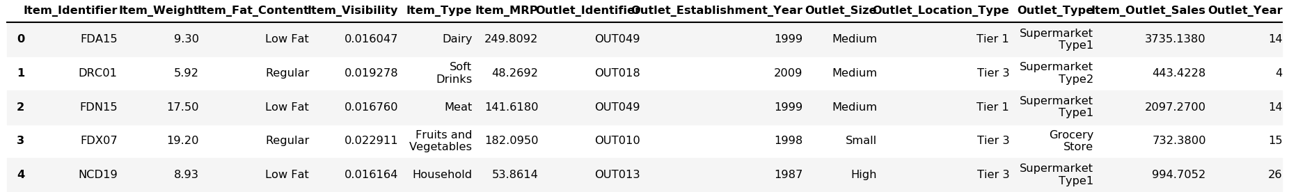

功能編碼 (Feature Encoding)

Encoding Categorical Variables

編碼分類變量

var_cat = train.select_dtypes(include=[object])
var_cat.head()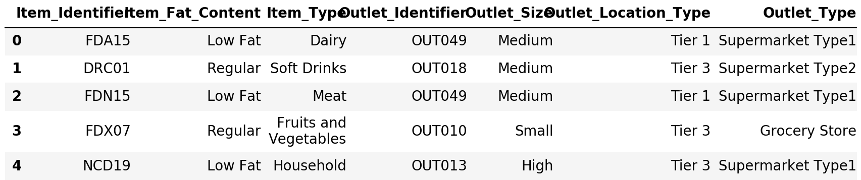

#Convert categorical into numerical 
var_cat = var_cat.columns.tolist()
var_cat = ['Item_Fat_Content',
 'Item_Type',
 'Outlet_Size',
 'Outlet_Location_Type',
 'Outlet_Type']
var_cat['Item_Fat_Content',
 'Item_Type',
 'Outlet_Size',
 'Outlet_Location_Type',
 'Outlet_Type']

Using Regex to rename the values in Item_type column and store it in a new column

使用Regex重命名Item_type列中的值并將其存儲在新列中

train.Item_Type_New.replace(to_replace="^FD*.*",value="Food",regex=True,inplace=True)train.Item_Type_New.replace(to_replace="^DR*.*",value="Drinks",regex=True,inplace=True)train.Item_Type_New.replace(to_replace="^NC*.*",value="Non-Consumable",regex=True,inplace=True)
train.head()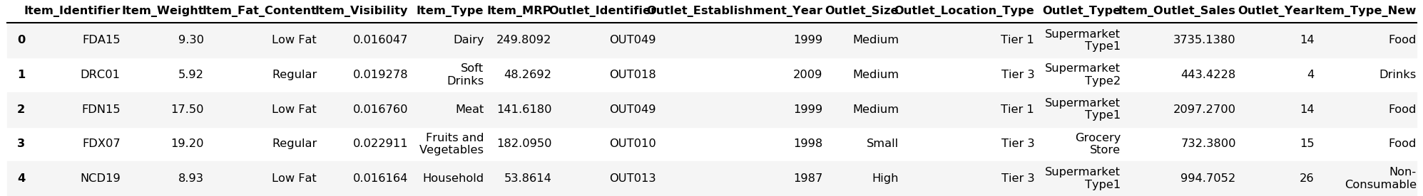

使用標簽編碼器的標簽編碼功能 (Label Encoding features using Label Encoder)

le = LabelEncoder()train['Outlet'] = le.fit_transform(train.Outlet_Identifier)
train['Item'] = le.fit_transform(train.Item_Type_New)
train.head()

for i in var_cat:
    train[i] = le.fit_transform(train[i])
train.head()

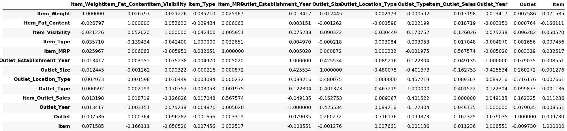
可視化相關 (Visualizing Correlation)

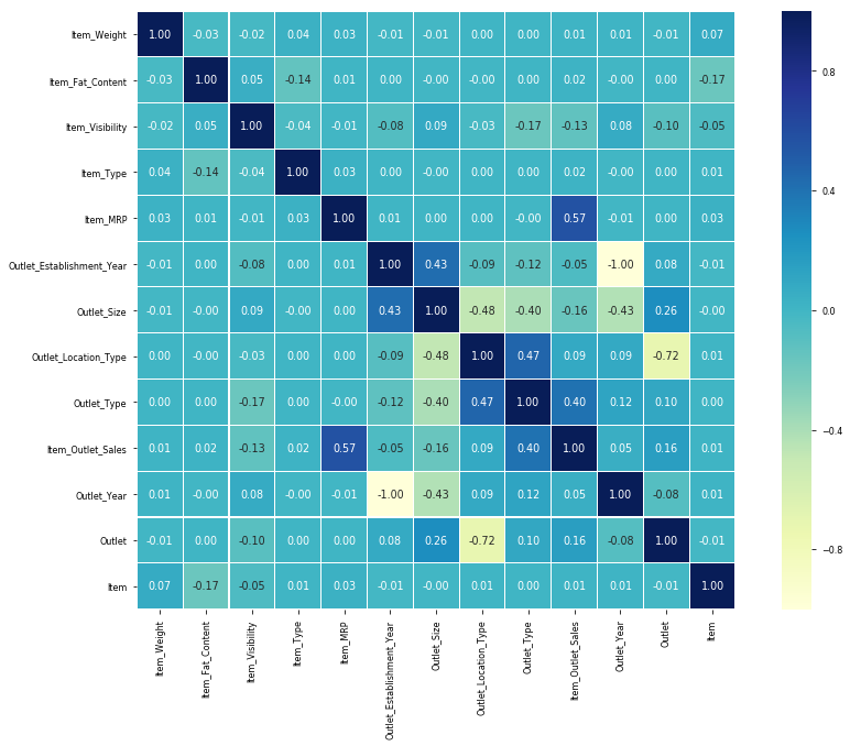
預測建模 (Predictive Modelling)

Choosing the predictors for our model

為我們的模型選擇預測因子

predictors=['Item_Fat_Content','Item_Visibility','Item_Type','Item_MRP','Outlet_Size','Outlet_Location_Type','Outlet_Type','Outlet_Year',
            'Outlet','Item','Item_Weight']
seed = 240
np.random.seed(seed)X = train[predictors]
y = train.Item_Outlet_SalesX.head()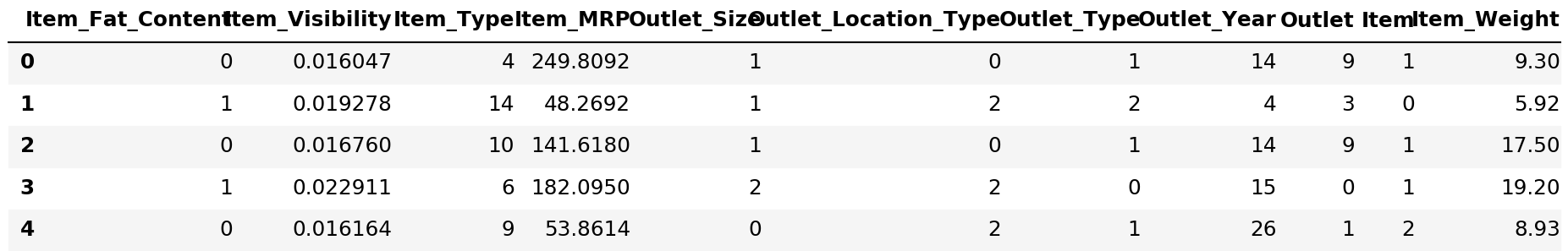

y.head()0    3735.1380
1     443.4228
2    2097.2700
3     732.3800
4     994.7052
Name: Item_Outlet_Sales, dtype: float64

將數據集分為訓練和測試數據 (Splitting the Dataset into Training and Testing Data)

X_train,X_test,y_train,y_test = train_test_split(X,y,test_size = 0.25,random_state = 42)X_train.shape(6392, 11)X_train.tail()

X_test.shape(2131, 11)y_train.shape(6392,)y_test.shape(2131,)

建筑模型 (Model Building)

We will be building different types of models.

我們將建立不同類型的模型。

1. Linear Regression
   線性回歸

lm = LinearRegression()model = lm.fit(X_train,y_train)
predictions = lm.predict(X_test)

繪制模型結果 (Plotting the model results)

plt.scatter(y_test,predictions)
plt.show()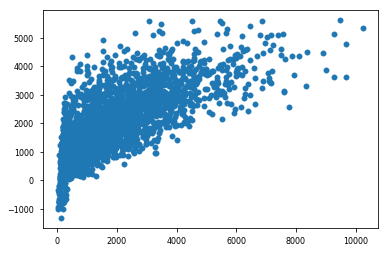

評估模型 (Evaluating the Model)

#R^2 Score
print("Linear Regression Model Score:",model.score(X_test,y_test))Linear Regression Model Score: 0.5052133696581114

計算RMSE (Calculating RMSE)

original_values = y_test#Root mean squared error
rmse = np.sqrt(metrics.mean_squared_error(original_values,predictions))print("Linear Regression RMSE: ", rmse)

Linear Regression without cross validation:

沒有交叉驗證的線性回歸：

Linear Regression R2 score: 0.505inear Regression RMSE: 1168.37

L inear Regression R2得分：0.505inear Regression RMSE：1168.37

# Linear Regression with statsmodels
x = sm.add_constant(X_train)
results = sm.OLS(y_train,x).fit()
results.summary()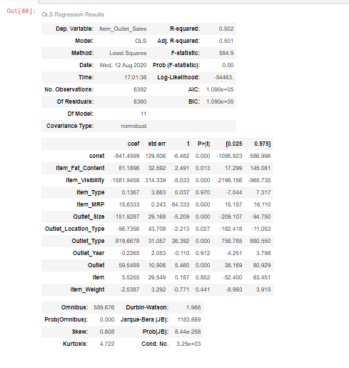

predictions = results.predict(x)predictionsDF = pd.DataFrame({"Predictions":predictions})
joined = x.join(predictionsDF)
joined.head()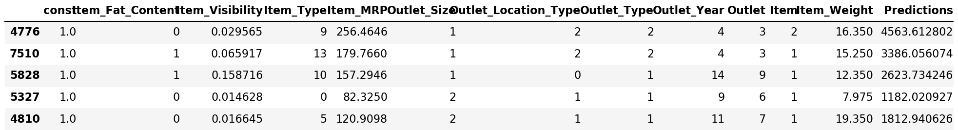

執行交叉驗證 (Performing Cross Validation)

# Perform 6-fold cross validation
score = cross_val_score(model,X,y,cv=5)
print("Linear Regression CV Score: ",score)

Linear Regression CV Score: [0.51828865 0.5023478 0.48262104 0.50311721 0.4998021 ]

線性回歸CV得分：[0.51828865 0.5023478 0.48262104 0.50311721 0.4998021]

Predicting with cross_val_predict

用cross_val_predict預測

predictions = cross_val_predict(model,X,y,cv=6)# Plotting the results
plt.scatter(y,predictions)
plt.show()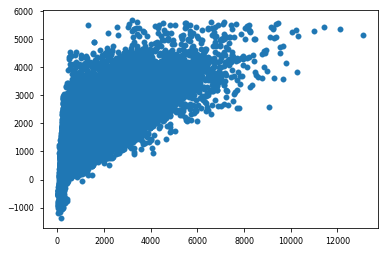

Linear Regression with Cross- Validation

具有交叉驗證的線性回歸

Linear Regression R2 with CV: 0.501inear Regression RMSE with CV: 1205.05

具有CV的L線性回歸R2： 0.501具有CV的線性回歸RMSE： 1205.05

使用KFold驗證 (Using KFold Validation)

Function to fit the model and return training and validation error

擬合模型并返回訓練和驗證錯誤的功能

def calc_metrics(X_train, y_train, X_test, y_test, model):
    '''fits model and returns the RMSE for in-sample error and out-of-sample error'''    model.fit(X_train, y_train)    train_error = calc_train_error(X_train, y_train, model)    validation_error = calc_validation_error(X_test, y_test, model)
    return train_error, validation_error

計算訓練誤差的功能 (Function to calculate the training error)

def calc_train_error(X_train, y_train, model):
    '''returns in-sample error for already fit model.'''
    predictions = model.predict(X_train)
    mse = metrics.mean_squared_error(y_train, predictions)
    rmse = np.sqrt(mse)
    return mse

Function to calculate the validation (Function to calculate the validation)

    
def calc_validation_error(X_test, y_test, model):
    '''returns out-of-sample error for already fit model.'''
    predictions = model.predict(X_test)
    mse = metrics.mean_squared_error(y_test, predictions)
    rmse = np.sqrt(mse)
    return mse

與Lasso回歸一起執行10倍交叉驗證，以克服模型的過擬合問題。 (Performing 10 fold Cross Validation along with Lasso Regression to overcome over-fitting of the model.)

Find the code here: CODE

在此處找到代碼： CODE

2.決策樹回歸器 (2. Decision Tree Regressor)

regressor = DecisionTreeRegressor(random_state=0)
regressor.fit(X_train,y_train)DecisionTreeRegressor(criterion='mse', max_depth=None, max_features=None,
           max_leaf_nodes=None, min_impurity_decrease=0.0,
           min_impurity_split=None, min_samples_leaf=1,
           min_samples_split=2, min_weight_fraction_leaf=0.0,
           presort=False, random_state=0, splitter='best')predictions = regressor.predict(X_test)
predictions[:5]array([ 792.302 ,  356.8688,  365.5242, 5778.4782, 2356.932 ])results = pd.DataFrame({'Actual':y_test,'Predicted':predictions})
results.head()

具有Kfold驗證的決策樹回歸 (Decision Tree Regression with Kfold validation)

Mean Absolute Error: 625.88Root Mean Squared Error: 1161.40

平均絕對誤差： 625.88均方根誤差： 1161.40

3.隨機森林回歸 (3. Random Forest Regressor)

Model that gave me the best RMSE

給我最好的RMSE的模型

rf = RandomForestRegressor(random_state=43)rf.fit(X_train,y_train)RandomForestRegressor(bootstrap=True, criterion='mse', max_depth=None,
           max_features='auto', max_leaf_nodes=None,
           min_impurity_decrease=0.0, min_impurity_split=None,
           min_samples_leaf=1, min_samples_split=2,
           min_weight_fraction_leaf=0.0, n_estimators=10, n_jobs=1,
           oob_score=False, random_state=43, verbose=0, warm_start=False)predictions = rf.predict(X_test)rmse = np.sqrt(metrics.mean_squared_error(y_test,predictions))results = pd.DataFrame({'Actual':y_test,'Predicted':predictions})
results.head()

具有kfold驗證得分的Randorm森林回歸 (Randorm Forest Regression with kfold validation score)

RMSE：946.34 R2得分：0.675 (RMSE: 946.34
R2 Score: 0.675)

摘要 (Summary)

This was a great learning project for me as I applied a lot of different techniques and researched a lot on different issues I faced throughout the duration of the project. I would like to thanks Analytics Vidhya team for hosting this challenge. Also, kudos to Towards Data Science for their amazing content on different aspects of Data Science.

對我來說，這是一個很棒的學習項目，因為我運用了許多不同的技術，并對整個項目期間遇到的不同問題進行了很多研究。 我要感謝Analytics Vidhya團隊承辦這項挑戰。 另外，對走向數據科學的榮譽 他們在數據科學各個方面的精彩內容。

未來的改進 (Future Improvements)

Hyper-parameter Tuning and Gradient Boosting.

超參數調整和梯度提升。