介紹 (Introduction)

Decision Trees (DTs) are a non-parametric supervised learning method used for classification and regression. The goal is to create a model that predicts the value of a target variable by learning simple decision rules inferred from the data features. Decision trees are commonly used in operations research, specifically in decision analysis, to help identify a strategy most likely to reach a goal, but are also a popular tool in machine learning.

決策樹(DT)是一種用于分類和回歸的非參數監督學習方法。 目標是創建一個模型，該模型通過學習從數據特征推斷出的簡單決策規則來預測目標變量的值。 決策樹通常用于運營研究中，尤其是決策分析中，用于幫助確定最有可能達成目標的策略，但它也是機器學習中的一種流行工具。

語境 (Context)

In this article, we will be discussing the following topics

在本文中，我們將討論以下主題

1. What are decision trees in general
   一般而言，決策樹是什么
2. Types of decision trees.
   決策樹的類型。
3. Algorithms used to build decision trees.
   用于構建決策樹的算法。
4. The step-by-step process of building a Decision tree.
   建立決策樹的分步過程。

什么是決策樹？ (What are Decision trees?)

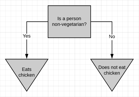
The above picture is a simple decision tree. If a person is non-vegetarian, then he/she eats chicken (most probably), otherwise, he/she doesn’t eat chicken. The decision tree, in general, asks a question and classifies the person based on the answer. This decision tree is based on a yes/no question. It is just as simple to build a decision tree on numeric data.

上圖是一個簡單的決策樹。 如果一個人不是素食者，那么他(她)很可能會吃雞肉，否則，他/她不會吃雞肉。 通常，決策樹會提出問題并根據答案對人員進行分類。 該決策樹基于是/否問題。 在數字數據上構建決策樹非常簡單。

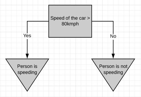
If a person is driving above 80kmph, we can consider it as over-speeding, else not.

如果一個人以每小時80英里的速度行駛，我們可以認為它是超速行駛，否則就不行。

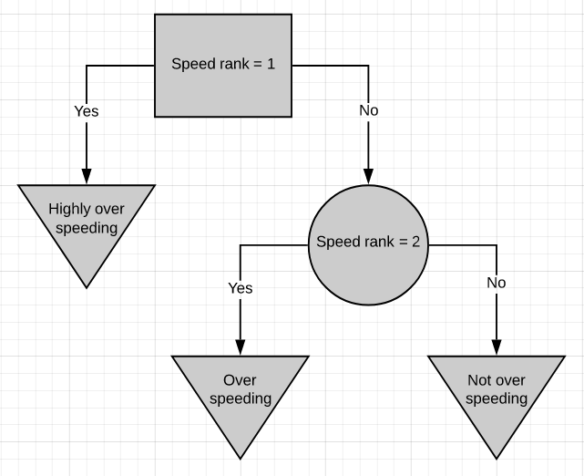
Here is one more simple decision tree. This decision tree is based on ranked data, where 1 means the speed is too high, 2 corresponds to a much lesser speed. If a person is speeding above rank 1 then he/she is highly over-speeding. If the person is above speed rank 2 but below speed rank 1 then he/she is over-speeding but not that much. If the person is below speed rank 2 then he/she is driving well within speed limits.

這是另一種簡單的決策樹。 該決策樹基于排名數據，其中1表示速度太高，2表示速度要低得多。 如果一個人超速超過等級1，那么他/她就極度超速。 如果此人在速度等級2以上但在速度等級1以下，則他/她超速，但不是那么多。 如果該人低于速度等級2，則他/她在速度限制內駕駛得很好。

The classification in a decision tree can be both categoric or numeric.

決策樹中的分類可以是分類的，也可以是數字的。

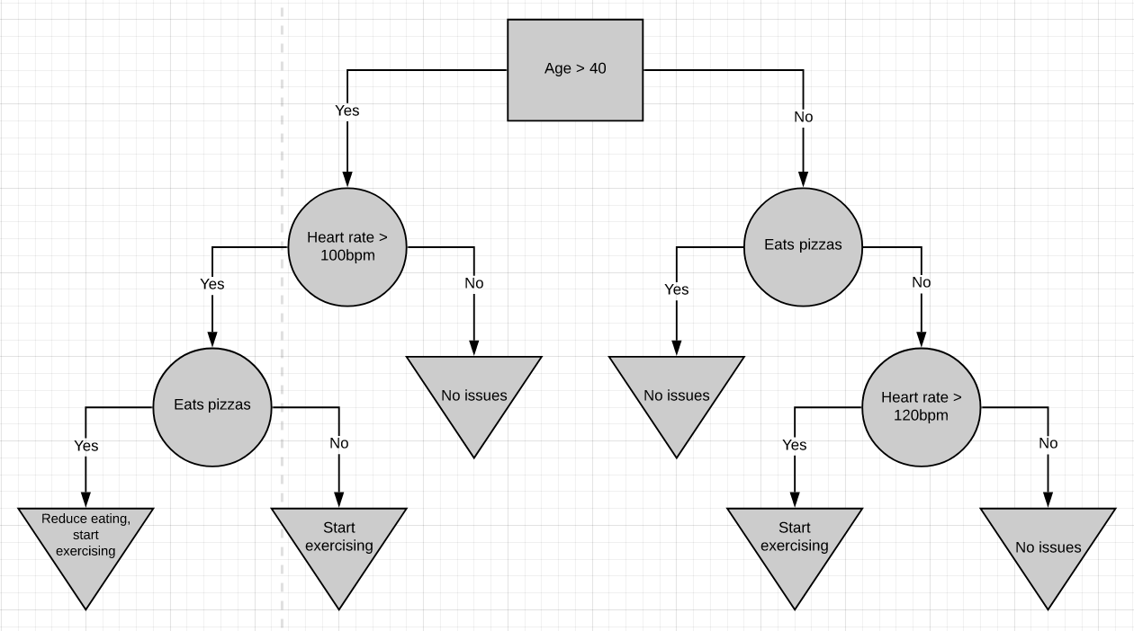
Here’s a more complicated decision tree. It combines numeric data with yes/no data. For the most part Decision trees are pretty simple to work with. You start at the top and work your way down till you get to a point where you cant go further. That’s how a sample is classified.

這是一個更復雜的決策樹。 它將數字數據與是/否數據組合在一起。 在大多數情況下，決策樹非常簡單。 您從頂部開始，一直往下走，直到到達無法繼續前進的地步。 這就是樣本分類的方式。

The very top of the tree is called the root node or just the root. The nodes in between are called internal nodes. Internal nodes have arrows pointing to them and arrows pointing away from them. The end nodes are called the leaf nodes or just leaves. Leaf nodes have arrows pointing to them but no arrows pointing away from them.

樹的最頂端稱為根節點 或只是根。 中間的節點稱為內部節點 。 內部節點具有指向它們的箭頭和指向遠離它們的箭頭。 末端節點稱為葉子節點或僅稱為葉子 。 葉節點有指向它們的箭頭，但沒有指向遠離它們的箭頭。

In the above diagrams, root nodes are represented by rectangles, internal nodes by circles, and leaf nodes by inverted-triangles.

在上圖中，根節點用矩形表示，內部節點用圓形表示，葉節點用倒三角形表示。

建立決策樹 (Building a Decision tree)

There are several algorithms to build a decision tree.

有幾種算法可以構建決策樹。

1. CART-Classification and Regression Trees
   CART分類和回歸樹
2. ID3-Iterative Dichotomiser 3
   ID3迭代二分頻器3
3. C4.5
   C4.5
4. CHAID-Chi-squared Automatic Interaction Detection
   CHAID卡方自動交互檢測

We will be discussing only CART and ID3 algorithms as they are the ones majorly used.

我們將僅討論CART和ID3算法，因為它們是最常用的算法。

大車 (CART)

CART is a DT algorithm that produces binary Classification or Regression Trees, depending on whether the dependent (or target) variable is categorical or numeric, respectively. It handles data in its raw form (no preprocessing needed) and can use the same variables more than once in different parts of the same DT, which may uncover complex interdependencies between sets of variables.

CART是一種DT算法，它分別根據因變量(或目標變量)是分類變量還是數字變量而生成二進制 分類樹或回歸樹。 它以原始格式處理數據(無需預處理)，并且可以在同一DT的不同部分中多次使用相同的變量，這可能揭示變量集之間的復雜相互依賴性。

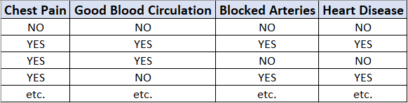
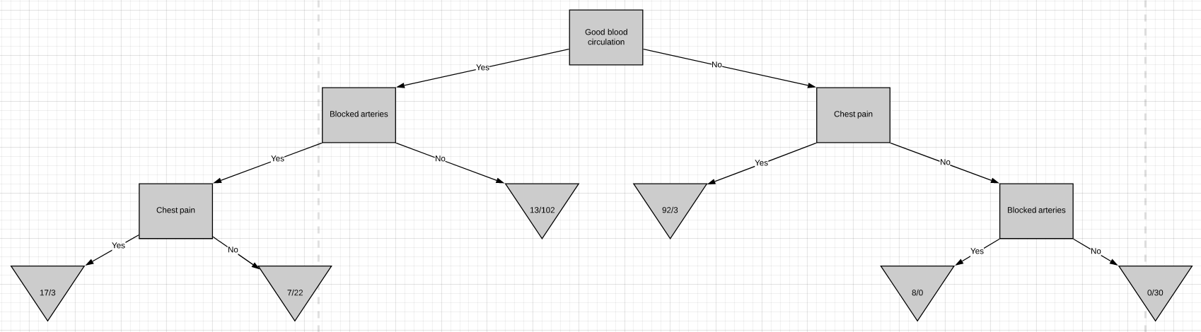
Now we are going to discuss how to build a decision tree from a raw table of data. In the example given above, we will be building a decision tree that uses chest pain, good blood circulation, and the status of blocked arteries to predict if a person has heart disease or not.

現在，我們將討論如何從原始數據表構建決策樹。 在上面給出的示例中，我們將構建一個決策樹，該決策樹使用胸痛，良好的血液循環以及動脈阻塞的狀態來預測一個人是否患有心臟病。

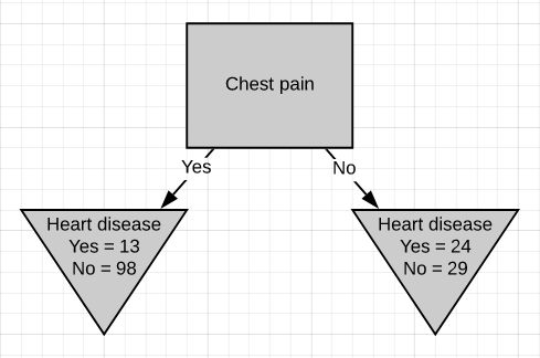
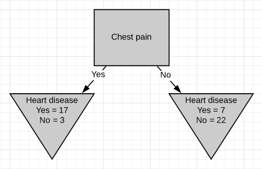
The first thing we have to know is which feature should be on the top or in the root node of the tree. We start by looking at how chest pain alone predicts heart disease.

我們首先要知道的是哪個功能應該在樹的頂部或根節點中。 我們首先來看僅胸痛是如何預示心臟病的。

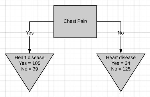
There are two leaf nodes, one each for the two outcomes of chest pain. Each of the leaves contains the no. of patients having heart disease and not having heart disease for the corresponding entry of chest pain. Now we do the same thing for good blood circulation and blocked arteries.

有兩個葉結，每個胸結分別導致兩種胸痛。 每片葉子都包含no。 患有心臟病而沒有心臟病的患者中，有相應的胸痛會進入。 現在，我們為血液循環良好和動脈阻塞做了同樣的事情。

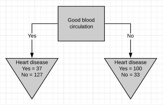
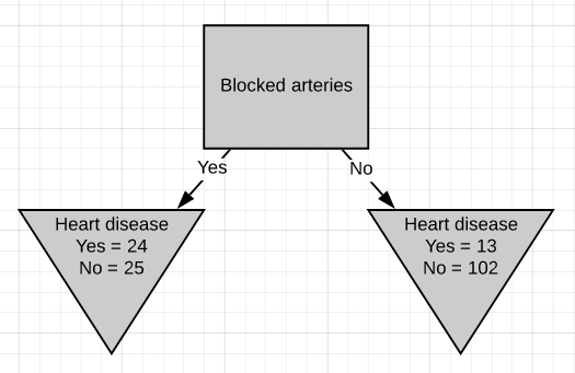
We can see that neither of the 3 features separates the patients having heart disease from the patients not having heart disease perfectly. It is to be noted that the total no. of patients having heart disease is different in all three cases. This is done to simulate the missing values present in real-world datasets.

我們可以看到，這三個特征都沒有將患有心臟病的患者與沒有患有心臟病的患者完美地分開。 要注意的是總數。 在這三種情況下，患有心臟病的患者的比例均不同。 這樣做是為了模擬現實數據集中存在的缺失值。

Because none of the leaf nodes is either 100% ‘yes heart disease’ or 100% ‘no heart disease’, they are all considered impure. To decide on which separation is the best, we need a method to measure and compare impurity.

因為所有葉節點都不是100％“是心臟病”或100％“沒有心臟病”，所以它們都被認為是不純的。 為了確定哪種分離最好，我們需要一種測量和比較雜質的方法。

The metric used in the CART algorithm to measure impurity is the Gini impurity score. Calculating Gini impurity is very easy. Let’s start by calculating the Gini impurity for chest pain.

CART算法中用于測量雜質的度量標準是基尼雜質評分 。 計算基尼雜質非常簡單。 讓我們從計算吉尼雜質引起的胸痛開始。

For the left leaf,

對于左葉

Gini impurity = 1 - (probability of ‘yes’)2 - (probability of ‘no’)2
              = 1 - (105/105+39)2 - (39/105+39)2
Gini impurity = 0.395

Similarly, calculate the Gini impurity for the right leaf node.

同樣，計算右葉節點的基尼雜質。

Gini impurity = 1 - (probability of ‘yes’)2 - (probability of ‘no’)2
              = 1 - (34/34+125)2 - (125/34+125)2
Gini impurity = 0.336

Now that we have measured the Gini impurity for both leaf nodes, we can calculate the total Gini impurity for using chest pain to separate patients with and without heart disease.

既然我們已經測量了兩個葉節點的Gini雜質，我們就可以計算出總的Gini雜質，使用胸部疼痛來區分患有和不患有心臟病的患者。

The leaf nodes do not represent the same no. of patients as the left leaf represents 144 patients and the right leaf represents 159 patients. Thus the total Gini impurity will be the weighted average of the leaf node Gini impurities.

葉節點不代表相同的編號。 的患者，因為左葉代表144位患者，右葉代表159位患者。 因此，總基尼雜質將是葉節點基尼雜質的加權平均值。

Gini impurity = (144/144+159)*0.395 + (159/144+159)*0.336
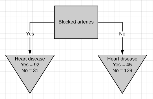
              = 0.364

Similarly the total Gini impurity for ‘good blood circulation’ and ‘blocked arteries’ is calculated as

同樣，“良好血液循環”和“動脈阻塞”的總基尼雜質計算如下：

Gini impurity for ‘good blood circulation’ = 0.360
Gini impurity for ‘blocked arteries’ = 0.381

‘Good blood circulation’ has the lowest impurity score among the tree which symbolizes that it best separates the patients having and not having heart disease, so we will use it at the root node.

“良好的血液循環”在樹中具有最低的雜質評分，這表示它可以最好地區分患有和不患有心臟病的患者，因此我們將在根結點使用它。

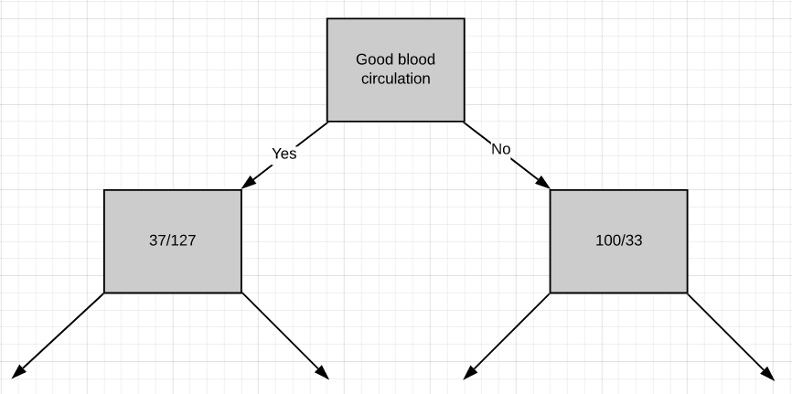
Now we need to figure out how well ‘chest pain’ and ‘blocked arteries’ separate the 164 patients in the left node(37 with heart disease and 127 without heart disease).

現在，我們需要弄清楚“胸痛”和“動脈阻塞”對左結的164例患者(37例有心臟病和127例無心臟病)的分隔情況。

Just like we did before we will separate these patients with ‘chest pain’ and calculate the Gini impurity value.

就像我們之前所做的那樣，我們將這些患有“胸痛”的患者分開，并計算出基尼雜質值。

The Gini impurity was found to be 0.3. Then we do the same thing for ‘blocked arteries’.

發現基尼雜質為0.3。 然后，我們對“阻塞的動脈”執行相同的操作。

The Gini impurity was found to be 0.29. Since ‘blocked arteries’ has the lowest Gini impurity, we will use it at the left node in Fig.10 for further separating the patients.

發現基尼雜質為0.29。 由于“阻塞的動脈”具有最低的基尼雜質，因此我們將在圖10的左側節點使用它來進一步分離患者。

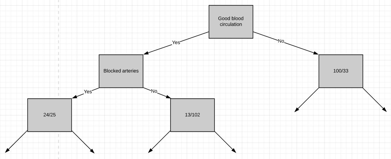
All we have left is ‘chest pain’, so we will see how well it separates the 49 patients in the left node(24 with heart disease and 25 without heart disease).

我們只剩下“胸痛”，因此我們將看到它如何很好地分隔了左結中的49位患者(24位有心臟病和25位無心臟病)。

We can see that chest pain does a good job separating the patients.

我們可以看到，胸痛在分隔患者方面做得很好。

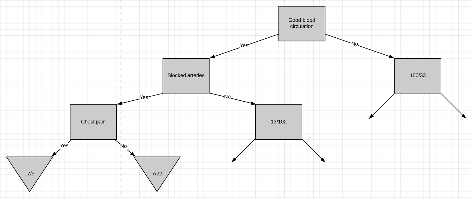
So these are the final leaf nodes of the left side of this branch of the tree. Now let’s see what happens when we try to separate the node having 13/102 patients using ‘chest pain’. Note that almost 90% of the people in this node are not having heart disease.

因此，這些是樹的此分支左側的最終葉節點。 現在，讓我們看看當嘗試使用“胸痛”分離具有13/102個患者的節點時會發生什么。 請注意，此節點中幾乎90％的人沒有心臟病。

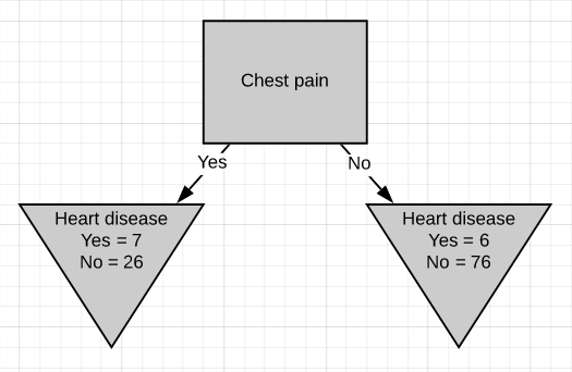
The Gini impurity of this separation is 0.29. But the Gini impurity for the parent-node before using chest-pain to separate the patients is

該分離的基尼雜質為0.29。 但是在使用胸痛將患者分開之前，父節點的基尼雜質是

Gini impurity = 1 - (probability of yes)2 - (probability of no)2
              = 1 - (13/13+102)2 - (102/13+102)2
Gini impurity = 0.2

The impurity is lower if we don’t separate patients using ‘chest pain’. So we will make it a leaf-node.

如果我們不使用“胸痛”將患者分開，那么雜質就更少。 因此，我們將其設為葉節點。

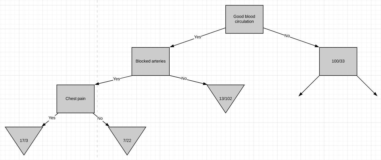
At this point, we have worked out the entire left side of the tree. The same steps are to be followed to work out the right side of the tree.

至此，我們已經算出了樹的整個左側。 遵循相同的步驟來計算樹的右側。

1. Calculate the Gini impurity scores.
   計算基尼雜質分數。
2. If the node itself has the lowest score, then there is no point in separating the patients anymore and it becomes a leaf node.
   如果節點本身的得分最低，則不再需要分離患者，而是成為葉節點。
3. If separating the data results in improvement then pick the separation with the lowest impurity value.
   如果分離數據可以改善質量，則選擇雜質值最低的分離方法。

ID3 (ID3)

The process of building a decision tree using the ID3 algorithm is almost similar to using the CART algorithm except for the method used for measuring purity/impurity. The metric used in the ID3 algorithm to measure purity is called Entropy.

除了用于測量純度/雜質的方法外，使用ID3算法構建決策樹的過程幾乎與使用CART算法相似。 ID3算法中用于測量純度的度量標準稱為熵 。

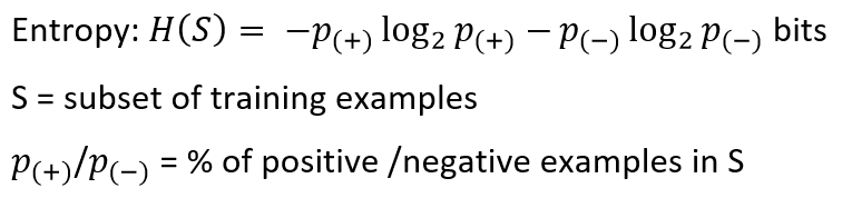
Entropy is a way to measure the uncertainty of a class in a subset of examples. Assume item belongs to subset S having two classes positive and negative. Entropy is defined as the no. of bits needed to say whether x is positive or negative.

熵是一種在子集中的示例中衡量類的不確定性的方法。 假設項屬于具有正負兩個類別的子集S。 熵定義為否。 需要說出x是正還是負的位。

Entropy always gives a number between 0 and 1. So if a subset formed after separation using an attribute is pure, then we will be needing zero bits to tell if is positive or negative. If the subset formed is having equal no. of positive and negative items then the no. of bits needed would be 1.

熵總是給出一個介于0和1之間的數字。因此，如果使用屬性進行分離后形成的子集是純凈的，那么我們將需要零位來判斷它是正還是負。 如果形成的子集具有相等的否。 積極和消極的項目，然后沒有。 需要的位數為1。

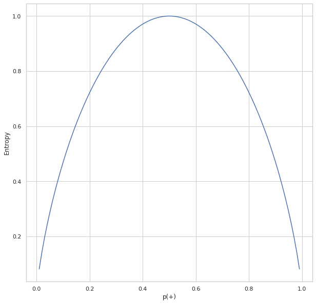
The above plot shows the relation between entropy and i.e., the probability of positive class. As we can see, the entropy reaches 1 which is the maximum value when which is there are equal chances for an item to be either positive or negative. The entropy is at its minimum when p(+) tends to zero(symbolizing x is negative) or 1(symbolizing x is positive).

上圖顯示了熵與正類別概率之間的關系。 正如我們所看到的，熵達到1時，這是最大值，當一個項目有相等的機會成為正數或負數時。 當p(+)趨于零(象征x為負)或1(象征x為正)時，熵處于最小值。

Entropy tells us how pure or impure each subset is after the split. What we need to do is aggregate these scores to check whether the split is feasible or not. This is done by Information gain.

熵告訴我們分割后每個子集的純或不純。 我們需要做的是匯總這些分數，以檢查拆分是否可行。 這是通過信息獲取來完成的。

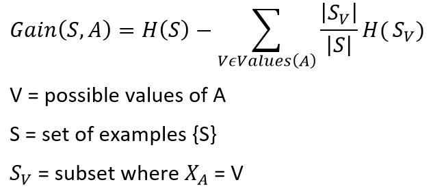
Consider this part of the problem we discussed above for the CART algorithm. We need to decide which attribute to use from chest pain and blocked arteries for separating the left node containing 164 patients(37 having heart disease and 127 not having heart disease). We can calculate the entropy before splitting as

考慮上面我們針對CART算法討論的問題的這一部分。 我們需要決定從chest pain和blocked arteries使用哪個屬性來分離左結，該左結包含164位患者(37位患有心臟病和127位沒有心臟病)。 我們可以在分解為

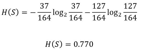
Let’s see how well chest pain separates the patients

讓我們看看chest pain如何使患者分開

The entropy for the left node can be calculated

可以計算出左節點的熵

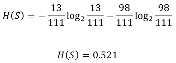
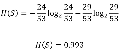
Similarly the entropy for the right node

類似地，右節點的熵

The total gain in entropy after splitting using chest pain

使用chest pain分裂后的總熵增加

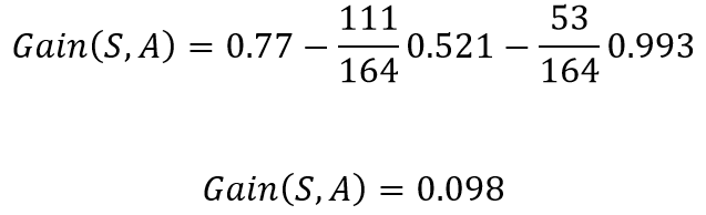
This implies that if in the current situation if we were to pick chest pain for splitting the patients, we would gain 0.098 bits in certainty on the patient having or not having heart disease. Doing the same for blocked arteries , the gain obtained was 0.117. Since splitting with blocked arteries gives us more certainty, it would be picked. We can repeat the same procedure for all the nodes to build a DT based on the ID3 algorithm.

這意味著，如果在當前情況下，如果我們為了讓患者分擔而chest pain ，那么在患有或沒有心臟病的患者中，我們將獲得0.098位的確定性。 對blocked arteries進行相同的操作，獲得的增益為0.117。 由于blocked arteries分裂 給我們更多的確定性，它將被選中。 我們可以對所有節點重復相同的過程，以基于ID3算法構建DT。

Note: The decision of whether to split a node into 2 or to declare it as a leaf node can be made by imposing a minimum threshold on the gain value required. If the acquired gain is above the threshold value, we can split the node, otherwise, leave it as a leaf node.

注意：通過將最小閾值強加在所需的增益值上，可以決定是將節點拆分為2還是將其聲明為葉節點。 如果獲取的增益高于閾值，則可以拆分節點，否則將其保留為葉節點。

摘要 (Summary)

The following are the take-aways from this article

以下是本文的摘錄

1. The general concept behind decision trees.
   決策樹背后的一般概念。
2. The basic types of decision trees.
   決策樹的基本類型。
3. Different algorithms to build a Decision tree.
   不同的算法來構建決策樹。
4. Building a Decision tree using CART algorithm.
   使用CART算法構建決策樹。
5. Building a Decision tree using ID3 algorithm.
   使用ID3算法構建決策樹。