For many years, academics have been using so-called frequentist statistics to evaluate whether experimental manipulations have significant effects.

多年以來，學者們一直在使用所謂的常客統計學來評估實驗操作是否具有significant效果。

Frequentist statistic is based on the concept of hypothesis testing, which is a mathematical based estimation of whether your results can be obtained by chance. The lower the value, the more significant it would be (in frequentist terms). By the same token, you can obtain non-significant results using the same approach. Most of these "negative" results are disregarded in research, although there is tremendous added value in also knowing what manipulations do not have an effect. But that’s for another post ;)

頻率統計基于假設檢驗的概念，假設檢驗是基于數學的估計，您是否可以偶然獲得結果。 值越低，它的意義就越大(以常用術語而言)。 同樣，您可以使用相同的方法獲得不重要的結果。 盡管大多數“負面”結果在了解什么操作沒有效果的過程中具有巨大的附加價值 ，但它們在研究中被忽略。 但這是另一篇文章;)

Thing is, in such cases where no effect can be found, frequentist statistics are limited in their explanatory power, as I will argue in this post.

事實是，在找不到效果的情況下，常客統計資料的解釋力受到限制，正如我將在本文中指出的那樣。

Below, I will be exploring one limitation of frequentist statistics, and proposing an alternative method to frequentist hypothesis testing: Bayesian statistics. I will not go into a direct comparison between the two approaches. There is quite some reading out there, if you are interested. I will rather explore how why the frequentist approach presents some shortcomings, and how the two approaches can be complementary in some situations (rather than seeing them as mutually exclusive, as sometimes argued).

下面，我將探討頻率論者統計的局限性，并提出一種用于頻率論者假設檢驗的替代方法： Bayesian統計。 我不會直接比較這兩種方法。 如果您有興趣的話，可以在這里讀很多書。 我寧愿探索為什么頻頻主義者的方法會帶來一些缺點，以及兩種方法在某些情況下如何互補(而不是像有時所說的那樣將它們視為互斥的)。

This is the first of two posts, where I will be focusing on the inability of frequentist statistics to disentangle between the absence of evidence and the evidence of absence.

這是兩篇文章中的第一篇，我將重點關注常客統計數據無法區分缺乏證據和缺乏證據之間的情況。

缺乏證據與缺乏證據 (Absence of evidence vs evidence of absence)

背景 (Background)

In the frequentist world, statistics typically output some statistical measures (t, F, Z values… depending on your test), and the almighty p-value. I discuss the limitations of only using p-values in another post, which you can read to get familiar with some concepts behind its computation. Briefly, the p-value, if significant (i.e., below an arbitrarily decided threshold, called alpha level, typically set at 0.05), determines that your manipulation most likely has an effect.

在常人世界中，統計數據通常會輸出一些統計量度(t，F，Z值……取決于您的測試)以及全能的p值。 我將在另一篇文章中討論僅使用p值的局限性，您可以閱讀以熟悉其計算背后的一些概念。 簡而言之，如果p值顯著(即低于任意確定的閾值，稱為alpha水平，通常設置為0.05)，則表明您的操作最有可能產生效果。

However, what if (and that happens a lot), your p-value is > 0.05? In the frequentist world, such p-values do not allow you to disentangle between an absence of evidence and an evidence of absence of effect.

但是，如果(而且經常發生)您的p值> 0.05怎么辦？ 在常識世界中，此類p值不允許您在缺乏證據和缺乏效果的證據之間做出區分。

Let that sink in for a little bit, because it is the crucial point here. In other words, frequentist statistics are pretty effective at quantifying the presence of an effect, but are quite poor at quantifying evidence for the absence of an effect. See here for literature.

讓它陷入一點，因為這是關鍵。 換句話說，頻繁出現的統計數據在量化效果存在方面非常有效，但在量化效果不存在的證據方面卻很差。 有關文學，請參見此處 。

The demonstration below is taken from some work that was performed at the Netherlands Institute for Neuroscience, back when I was working in neuroscience research. A very nice paper was recently published on this topic, that I encourage you to read. The code below is inspired by the paper repository, written in R.

下面的演示摘自我在神經科學研究領域工作時在荷蘭神經科學研究所所做的一些工作。 最近發表了一篇關于該主題的非常好的論文 ，我鼓勵您閱讀。 以下代碼受R編寫的紙質存儲庫的啟發。

模擬數據 (Simulated Data)

Say we generate a random distribution with mean=0.5 and standard deviation=1.

假設我們生成一個均值= 0.5和標準差= 1的隨機分布。

np.random.seed(42)
mean = 0.5; sd=1; sample_size=1000
exp_distibution = np.random.normal(loc=mean, scale=sd, size=sample_size)
plt.hist(exp_distibution)

That would be our experimental distribution, and we want to know whether that distribution is significantly different from 0. We could run a one sample t-test (which would be okay since the distribution seems very Gaussian, but you should theoretically prove that parametric testing assumptions are fulfilled; let’s assume they are)

那將是我們的實驗分布，我們想知道該分布是否與0顯著不同。我們可以運行一個樣本t檢驗(因為分布看起來非常高斯，所以可以，但是理論上您應該證明參數測試滿足假設；讓我們假設它們是)

t, p = stats.ttest_1samp(a=exp_distibution, popmean=0)
print(‘t-value = ‘ + str(t))
print(‘p-value = ‘ + str(p))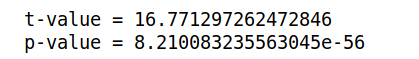

Quite a nice p-value that would make every PhD student’s spine shiver with happiness ;) Note that with that kind of sample size, almost anything gets significant, but let’s move on with the demonstration.

相當不錯的p值會使每個博士生都對幸福感顫抖；)請注意，使用這種樣本量，幾乎所有東西都變得很重要，但讓我們繼續進行演示。

Now let’s try a distribution centered at 0, which should not be significantly different from 0

現在，讓我們嘗試以0為中心的分布，該分布與0的差別應該不大

mean = 0; sd=1; sample_size=1000
exp_distibution = np.random.normal(loc=mean, scale=sd, size=sample_size)
plt.hist(exp_distibutiont, p = stats.ttest_1samp(a=exp_distibution, popmean=0)
print(‘t-value = ‘ + str(t))
print(‘p-value = ‘ + str(p))

Here, we have as expected a distribution that does not significantly differ from 0. And here is where things get a bit tricky: in some situations, frequentist statistics cannot really tell whether a p-value > 0.05 is an absence of evidence, and an evidence for absence, although that is a crucial point that would allow you to completely rule out an experimental manipulation from having an effect.

在這里，我們期望的分布與0的差異不大。在這里，情況變得有些棘手：在某些情況下，常客統計學不能真正判斷p值> 0.05是否缺少證據，而缺席的證據，盡管這是至關重要的一點，可以讓您完全排除實驗性操作的影響。

Let’s take an hypothetical situation:

讓我們假設一個情況：

You want to know whether a manipulation has an effect. It might be a novel marketing approach in your communication, a interference with biological activity or a “picture vs no picture” test in a mail you are sending. You of course have a control group to compare your experimental group to.

您想知道操作是否有效。 這可能是您交流中的一種新穎的營銷方式，是對生物活動的干擾，也可能是您發送的郵件中的“圖片與無圖片”測試。 您當然有一個對照組來比較您的實驗組。

When collecting your data, you could see different patterns:

收集數據時，您會看到不同的模式：

• (i) the two groups differ.
  (i)兩組不同。
• (ii) the two groups behave similarly.
  (ii)兩組的行為相似。
• (iii) you do not have enough observations to conclude (sample size too small)
  (iii)您沒有足夠的觀察結論(樣本量太小)

While option (i) is an evidence against the null hypothesis H0 (i.e., you have evidence that your manipulation had an effect), situations (ii) (=evidence for H0, i.e, evidence of absence) and (iii) (=no evidence, i.e, absence of evidence) cannot be disentangled using frequentist statistics. But maybe the bayesian approach can add something to this story...

盡管選項(i)是針對null hypothesis H0的證據(即，您有證據證明您的操縱有效果)，但情況(ii)(= H0的證據，即不存在的證據)和(iii)(=否)證據，即沒有證據)不能使用常客統計來弄清。 但是也許貝葉斯方法可以為這個故事增添些...

p值如何受效應和樣本量影響 (How p-values are affected by effect and sample sizes)

The first thing is to illustrate the situations where frequentist statistics have shortcomings.

首先是要說明常客統計數據存在缺陷的情況。

方法背景 (Approach background)

What I will be doing is plotting how frequentist p-values behave when changing both effect size (i.e., the difference between your control, here with a mean=0, and your experimental distributions) and sample size (number of observations or data points).

我要做的是繪制同時更改效果大小 (即，控件的均值= 0和實驗分布之間的差異)和樣本大小 (觀察值或數據點的數量)時，頻繁P值的行為。

Let’s first write a function that would compute these p-values:

讓我們首先編寫一個可以計算這些p值的函數：

def run_t_test(m,n,iterations):
    """
    Runs a t-test for different effect and sample sizes and stores the p-value
    """
    my_p = np.zeros(shape=[1,iterations])
    for i in range(0,iterations):
        x = np.random.normal(loc=m, scale=1, size=n)
        # Traditional one tailed t test
        t, p = stats.ttest_1samp(a=x, popmean=0)
        my_p[0,i] = p
    return my_p

We can then define the parameters of the space we want to test, with different sample and effect sizes:

然后，我們可以使用不同的樣本和效果大小來定義要測試的空間的參數：

# Defines parameters to be tested
sample_sizes = [5,8,10,15,20,40,80,100,200]
effect_sizes = [0, 0.5, 1, 2]
nSimulations = 1000

We can finally run the function and visualize:

我們最終可以運行該函數并進行可視化：

# Run the function to store all p-values in the array "my_pvalues"
my_pvalues = np.zeros((len(effect_sizes), len(sample_sizes),nSimulations))for mi in range(0,len(effect_sizes)):
    for i in range(0, len(sample_sizes)):
        my_pvalues[mi,i,] = run_t_test(m=effect_sizes[mi], 
                                n=sample_sizes[i], 
                                iterations=nSimulations
                               )

I will quickly visualize the data to make sure that the p-values seem correct. The output would be:

我將快速可視化數據以確保p值看起來正確。 輸出為：

p-values for sample size = 5
Effect sizes:
          0       0.5       1.0         2
0  0.243322  0.062245  0.343170  0.344045
1  0.155613  0.482785  0.875222  0.152519
p-values for sample size = 15
Effect sizes:
          0       0.5       1.0             2
0  0.004052  0.010241  0.000067  1.003960e-08
1  0.001690  0.000086  0.000064  2.712946e-07

I would make two main observations here:

我將在這里做兩個主要觀察：

1. When you have high enough sample size (lower section), the p-values behave as expected and decrease with increasing effect sizes (since you have more robust statistical power to detect the effect).
   當樣本量足夠大時(下半部分)，p值將按預期表現，并隨著效果大小的增加而減小(因為您有更強大的統計能力來檢測效果)。
2. However, we also see that the p-values are not significant for a small sample sizes, even if the effect sizes are quite large (upper section). That is quite striking, since the effect sizes are the same, only the number of data points is different.
   但是，我們也看到即使樣本量很大(上半部分)，p值對于小樣本量也并不重要。 這是非常驚人的，因為效果大小相同，所以只有數據點的數量不同。

Let’s visualize that.

讓我們想象一下。

可視化 (Visualization)

For each sample size (5, 8, 10, 15, 20, 40, 80, 100, 200), we will count the number of p-values falling in significance level bins.

對于每個樣本大小(5、8、10、15、20、40、80、100、200)，我們將計算落入顯著性等級箱中的p值的數量。

Let’s first compare two distributions of equal mean, that is, we have an effect size = 0.

讓我們首先比較兩個均值相等的分布，即我們的效果大小= 0。

As we can see from the plot above, most of the p-values computed by the t-test are not significant for an experimental distribution of mean 0. That makes sense, since these two distributions are not different in their means.

從上圖可以看出，通過t檢驗計算出的大多數p值對于平均值為0的實驗分布而言并不重要。這是有道理的，因為這兩種分布的均值沒有差異。

We can, however, see that in some cases, we do obtain significant p values, which can happen when using very particular data points drawn from the overall population. These are typically false positive, and the reason why it is important to repeat experiments and replicate results ;)

但是，我們可以看到，在某些情況下，我們確實獲得了顯著的p值，當使用從總體總體中得出的非常特殊的數據點時，可能會發生這種情況。 這些通常都是假陽性，是重復實驗和復制結果很重要的原因；)

Let’s see what happens if we use a distribution whose mean differs by 0.5 compared to the control:

讓我們看看如果我們使用與控件相比均值相差0.5的分布會發生什么：

Now, we clearly see that increasing sample size dramatically increases the ability to detect the effect, with still many non significant p-values for low sample sizes.

現在，我們清楚地看到，增加樣本量會極大地提高檢測效果的能力，但對于低樣本量，仍有許多不重要的p值。

Below, as expected, you see that for highly different distributions (effect size = 2), the number of significant p-values increase:

如下所示，可以看到，對于高度不同的分布(效果大小= 2)，有效p值的數量增加：

OK, so that was it for an illustrative example of how p-values are affected by sample and effect sizes.

好的，那是一個示例性示例，說明p值如何受樣本和效果大小影響。

Now, the problem is that when you have a non significant p value, you are not always sure whether you might have missed the effect (say because you had a low sample size, due to limited observations or budget) or whether your data really suggest the absence of an effect. As matter of fact, most scientific research have a problem of statistical power, because they have limited observations (due to experimental constraints, budget, time, publishing time pressure, etc…).

現在的問題是，當您的p值不顯著時，您將無法始終確定是否可能錯過了效果(例如，由于觀察或預算有限，樣本量較小)還是您的數據確實暗示了沒有效果。 實際上，大多數科學研究都有統計能力的問題，因為它們的觀察力有限(由于實驗限制，預算，時間，出版時間壓力等)。

Since the reality of data in research is a rather low sample size, you still might want to draw meaningful conclusions from non significant results based on low sample sizes.

由于研究中數據的真實性相當低，因此您可能仍想根據低樣本量從不重要的結果中得出有意義的結論。

Here, Bayesian statistics could help you make one more step with your data ;)

在這里，貝葉斯統計信息可以幫助您在數據處理方面邁出新一步；)

Stay tuned for the following post where I explore the Titanic and Boston data sets to demonstrate how Bayesian statistics can be useful in such cases!

請繼續關注以下文章，在該文章中我將探索泰坦尼克號和波士頓的數據集，以證明貝葉斯統計量在這種情況下如何有用！

You can find this notebook in the following repo: https://github.com/juls-dotcom/bayes

您可以在以下回購中找到此筆記本： https : //github.com/juls-dotcom/bayes