vc6.0 繪制散點圖
Scatterplots are one of the most popular visualization techniques in the world. Its purposes are recognizing clusters and correlations in ‘pairs’ of variables. There are many variations of scatter plots. We will look at some of them.
散點圖是世界上最流行的可視化技術之一。 其目的是識別變量“對”中的聚類和相關性。 散點圖有很多變體。 我們將研究其中的一些。
Strip Plots
帶狀圖
Scatter plots in which one attribute is categorical are called ‘strip plots’. Since it is hard to see the data points when we plot the data points as a single line, we need to slightly spread the data points, you can check the above and we can also divide the data points based on the given label.
其中一種屬性是分類的散點圖稱為“條形圖”。 由于在將數據點繪制為單線時很難看到數據點,因此我們需要稍微散布數據點,您可以檢查上述內容,也可以根據給定的標簽劃分數據點。
Scatterplot Matrices (SPLOM)
散點圖矩陣(SPLOM)
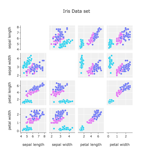
SPLOM produce scatterplots for all pairs of variables and place them into a matrix. Total unique scatterplots are (p2-p)/2. The diagonal is filled with KDE or histogram most of the time. As you can see, there is an order of scatterplots. Does the order matter? It cannot affect the value of course but it can affect the perception of people.
SPLOM為所有變量對生成散點圖,并將它們放入矩陣中。 總唯一散點圖為(p2-p)/ 2。 對角線大部分時間都充滿KDE或直方圖。 如您所見,有一個散點圖順序。 順序重要嗎? 它不會影響課程的價值,但會影響人們的感知。

Therefore we need to consider the order of it. Peng suggests the ordering that similar scatterplots are located close to each other in his work in 2004 [Peng et al. 2004]. They distinguish between high-cardinality and low cardinality(number of possible values > number of points means high cardinality.) and sort low-cardinality by a number of values. They rate the ordering of high-cardinality dimensions based on their correlation. Pearson Correlation Coefficient is used for sorting.
因此,我們需要考慮它的順序。 Peng建議在2004年的工作中將相似的散點圖放置在彼此附近的順序[Peng等。 2004]。 它們區分高基數和低基數(可能值的數量>點數表示高基數),并通過多個值對低基數進行排序。 他們根據它們的相關性對高基數維度的排序進行評分。 皮爾遜相關系數用于排序。

We find all other pairs of x,y scatter plots with clutter measure. It calculates all correlation and compares it with each pair (x,y ) of high-cardinality dimensions. If its results are smaller than the threshold we choose that scatter plot as an important one. However, it takes a lot of computing power because its big-o-notation is O(p2 * p!). They suggest random swapping, it chooses the smallest one and keeps it and again and again.
我們發現所有其他對具有散亂度量的x,y散點圖。 它計算所有相關并將其與高基數維的每對(x,y)進行比較。 如果其結果小于閾值,則選擇該散點圖作為重要散點圖。 但是,由于它的big-o表示法是O(p2* p!),因此需要大量的計算能力。 他們建議隨機交換,它選擇最小的交換并一次又一次地保留。
Selecting Good Views
選擇好的觀點
Correlation is not enough to choose the nice scatterplots when we are trying to find out the cluster based on the given label or we can get the label from clustering.
當我們嘗試根據給定標簽找出聚類時,或者僅從聚類中獲取標簽時,相關性不足以選擇合適的散點圖。
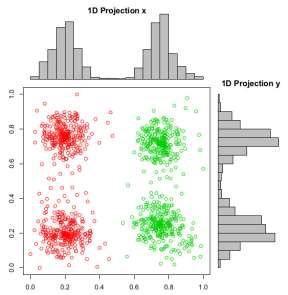
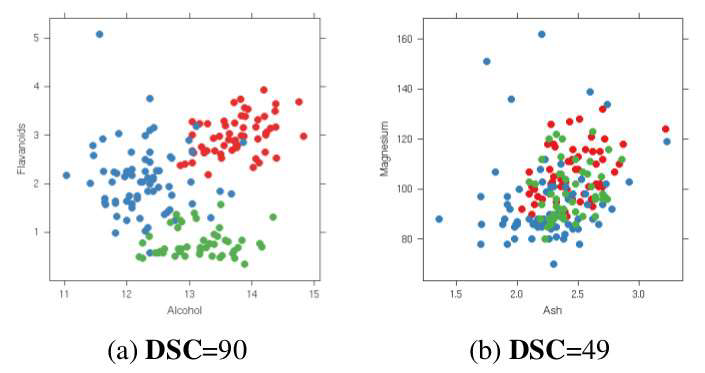
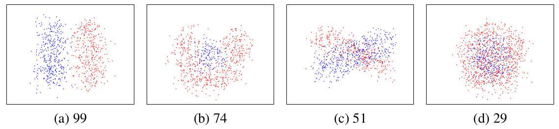
If you don’t have given labels in the left graph, you can pick x-axis projection or y-axis projection because there are no many differences but there are labels. Therefore, we can know the x-axis projection is correct., DSC is introduced with respect to this view that the method checks how good our scatterplot is. More good separation, more good scatterplots.
如果在左圖中沒有給出標簽,則可以選擇x軸投影或y軸投影,因為它們之間沒有太多差異,但是有標簽。 因此,我們可以知道x軸投影是正確的。為此,介紹了DSC,該方法檢查了散點圖的質量。 更好的分離,更好的散點圖。
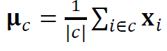
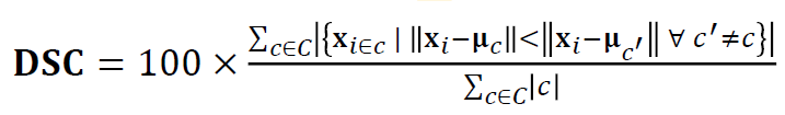
First of all, we calculate the center of each cluster and measure the distance between each data point and each cluster center. If the distance from its own cluster is shorter than other clusters distance, we increase the cardinality and we normalized it by the number of clusters and multiply 100. This method is similar to the k-means clustering method. Since it only considers distance, it has a limitation to applying.
首先,我們計算每個聚類的中心并測量每個數據點與每個聚類中心之間的距離。 如果距其自身群集的距離短于其他群集的距離,我們將增加基數,并通過群集數對其進行歸一化并乘以100。此方法類似于k均值群集方法。 由于僅考慮距離,因此在應用方面存在局限性。
Distribution Consistency (DC)
分配一致性(DC)
DC is the upgrade(?) version of DSC. DC measures the score based on penalizing local entropy in high-density regions. DSC assumes the particular cluster shapes but DC does not assume the shapes.
DC是DSC的升級版本。 DC基于懲罰高密度區域中的局部熵來測量分數。 DSC假定特定的群集形狀,但DC不假定這些形狀。
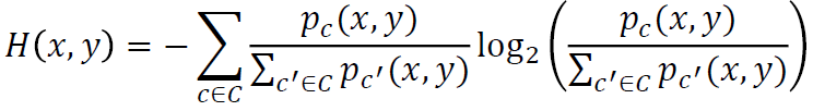
This equation is from information theory and it considers how much information in a specific distribution. The data should be estimated using KDE before we apply the entropy function, p(x,y) means the KDE. This equation means it gives smaller(Look at the minus) when the region we measure is mixed with other clusters and its minimum is 0 and the maximum is log2|C|.
該方程式來自信息理論,它考慮特定分布中有多少信息。 在應用熵函數之前,應使用KDE估算數據,p(x,y)表示KDE。 該方程式意味著當我們測量的區域與其他簇混合且其最小值為0且最大值為log2 | C |時,它的值較小(看一下負值)。
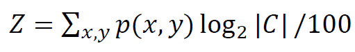
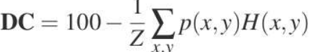
We calculated the entropy with KDE and we don’t want to calculate the whole region at the same weight because there are many vacant regions. Finally, we normalize the results. This gives the DC score. We can choose scatterplots based on thresholds that we can choose.
我們使用KDE來計算熵,我們不想以相同的權重來計算整個區域,因為有許多空置區域。 最后,我們將結果標準化。 這給出了DC得分。 我們可以根據選擇的閾值來選擇散點圖。
This dataset is from the WHO, 194 countries, 159 attributes, and 6 HIV risk groups. They focus on DC > 80 and they can eliminate 97% of the plots. It is a highly efficient method.
該數據集來自WHO,194個國家,159個屬性和6個HIV風險組。 他們專注于DC> 80,并且可以消除97%的地塊。 這是一種高效的方法。
Other than these methods that it only considers the clusters, there are many ways to consider other specific patterns, e.g. fraction of outliers, sparsity, convexity, and e.t.c. You can take a look at [Wilkinson et al. 2006]. PCA also can be used as an alternative way to group similar plots together.
除了僅考慮聚類的這些方法以外,還有許多方法可以考慮其他特定模式,例如,異常值的分數,稀疏性,凸度等。您可以看一下[Wilkinson等。 2006]。 PCA也可以用作將相似地塊組合在一起的替代方法。
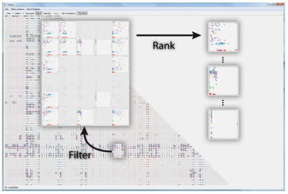
SPLOM Navigation
SPLOM導航

Since the SPLOM shares one axis with the neighboring plots, it is possible to project on to 3D space.
由于SPLOM與相鄰的圖共享一個軸,因此可以投影到3D空間。
The limitation of scatterplots: Overdraw
散點圖的局限性:透支

Too many data points lead to overdraw. We can solve this with KDE but it becomes no longer see individual points. The second problem is high dimensional data because it gives too many scatterplots. We discussed the solution of the second problem. Now we are going to look at the first problem.
太多的數據點導致透支。 我們可以使用KDE解決此問題,但不再看到單個點。 第二個問題是高維數據,因為它提供了太多的散點圖。 我們討論了第二個問題的解決方案。 現在我們要看第一個問題。
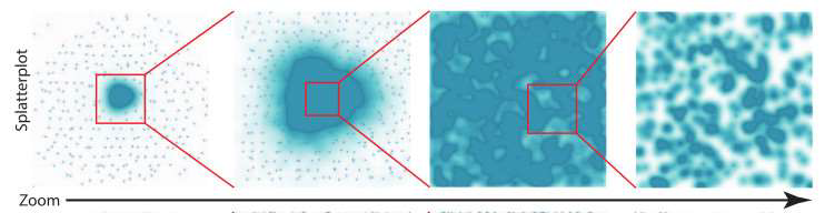
Splatterplots
飛濺圖

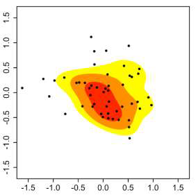
Splatterplots properly combine the KDE and Scatterplots. The high-density region is represented by colors and the low-density region is represented by a single data point. We need to choose a proper kernel width for KDE. Splatterplots define the kernel width in screen space, how many data points in the unit screen space. However, we need to choose the threshold by ourselves.
Splatterplots正確地將KDE和Scatterplots結合在一起。 高密度區域由顏色表示,低密度區域由單個數據點表示。 我們需要為KDE選擇合適的內核寬度。 Splatterplots定義屏幕空間中的內核寬度,即單位屏幕空間中有多少個數據點。 但是,我們需要自己選擇閾值。
If clusters are mixed, then colors are matter. High luminance and saturation can cause the miss perception that people can recognize the mixed cluster as a different cluster. Therefore, we need to reduce the saturation and luminance to indicate it is mixed clusters.
如果群集混合在一起,那么顏色就很重要。 高亮度和飽和度可能會導致人們誤以為人們會將混合群集識別為另一個群集。 因此,我們需要降低飽和度和亮度以表明它是混合簇。
This post is published on 9/2/2020.
此帖發布于2020年9月2日。
翻譯自: https://medium.com/@jeheonpark93/vc-everything-about-scatter-plots-467f80aec77c
vc6.0 繪制散點圖
本文來自互聯網用戶投稿,該文觀點僅代表作者本人,不代表本站立場。本站僅提供信息存儲空間服務,不擁有所有權,不承擔相關法律責任。 如若轉載,請注明出處:http://www.pswp.cn/news/389587.shtml 繁體地址,請注明出處:http://hk.pswp.cn/news/389587.shtml 英文地址,請注明出處:http://en.pswp.cn/news/389587.shtml
如若內容造成侵權/違法違規/事實不符,請聯系多彩編程網進行投訴反饋email:809451989@qq.com,一經查實,立即刪除!相關文章

sudo配置臨時取得root權限

Pytorch中RNN入門思想及實現

小扎不哭!FB又陷數據泄露風波,9000萬用戶受影響

在衡量歐洲的政治意識形態時,調查規模的微小變化可能會很重要

Pytorch中CNN入門思想及實現

java常用設計模式一:單例模式

SDUT-2121_數據結構實驗之鏈表六:有序鏈表的建立

事件映射 消息映射_映射幻影收費站


Pytorch中BN層入門思想及實現

JDK源碼學習筆記——TreeMap及紅黑樹

匿名內部類和匿名類_匿名schanonymous

Pytorch框架中SGD&Adam優化器以及BP反向傳播入門思想及實現

朱曄和你聊Spring系列S1E3:Spring咖啡罐里的豆子

ab實驗置信度_為什么您的Ab測試需要置信區間

基于Pytorch的NLP入門任務思想及代碼實現:判斷文本中是否出現指定字
方法源碼解析(二))
erlang下lists模塊sort(排序)方法源碼解析(二)
)
洛谷P4841 城市規劃(多項式求逆)

支撐阻力指標_使用k表示聚類以創建支撐和阻力
python在anaconda安裝opencv庫及skimage庫(scikit_image庫)諸多問題解決辦法)