Churn prediction, namely predicting clients who might want to turn down the service, is one of the most common business applications of machine learning. It is especially important for those companies providing streaming services. In this project, an event data set from a fictional music streaming company named Sparkify was analyzed. A tiny subset (128MB) of the full dataset (12GB) was first analyzed locally in Jupyter Notebook with a scalable script in Spark and the whole data set was analyzed on the AWS EMR cluster. Find the code here.

流失預測(即預測可能要拒絕服務的客戶)是機器學習最常見的業務應用之一。 對于提供流媒體服務的公司而言，這一點尤其重要。 在該項目中，分析了一家虛構的音樂流媒體公司Sparkify的事件數據集。 首先在Jupyter Notebook中使用Spark中的可擴展腳本在本地對整個數據集(12GB)的一小部分(128MB)進行分析，然后在AWS EMR集群上分析整個數據集。 在此處找到代碼。

資料準備 (Data preparation)

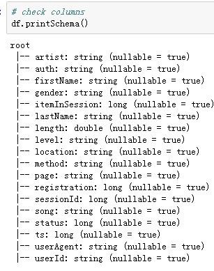
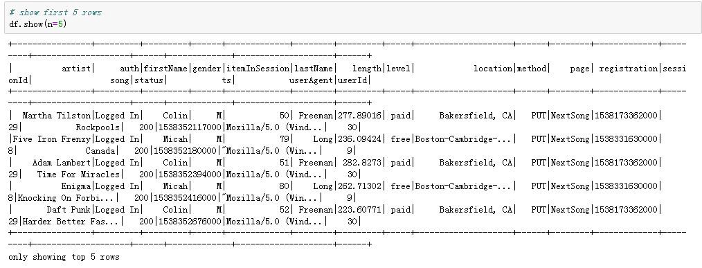
Let’s first have a look at the data. There were 286500 rows and 18 columns in the mini data set (in the big data set, there were 26259199 rows). The columns and first five rows were shown as follows.

首先讓我們看一下數據。 小型數據集中有286500行和18列(在大數據集中有26259199行)。 列和前五行如下所示。

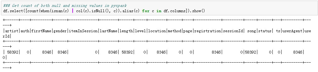
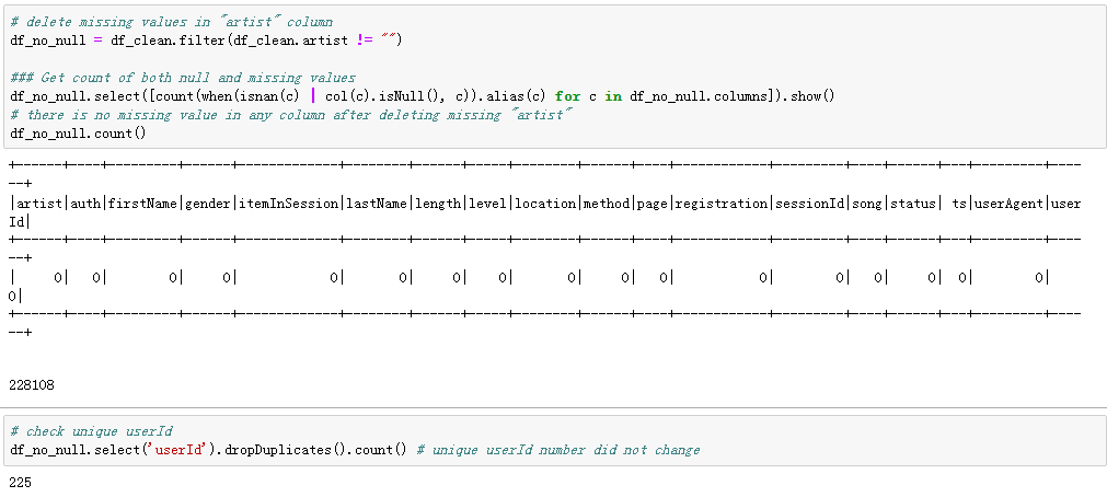
Let’s check missing values in the data set. We will find a pattern from the table below in the missing values: There was the same number of missing values in the “artist”,” length”, and the ”song” columns, and the same number of missing values in the “firstName”, “gender”, “lastName”, “location”,” registration”, and ”userAgent” columns.

讓我們檢查數據集中的缺失值。 我們將從下表中找到缺失值的模式：“藝術家”，“長度”和“歌曲”列中缺失值的數量相同，而“名字”中缺失值的數量相同”，“性別”，“姓氏”，“位置”，“注冊”和“ userAgent”列。

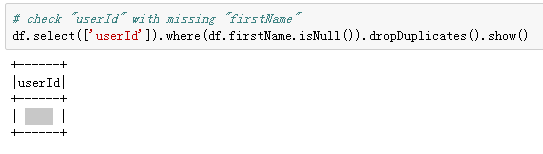
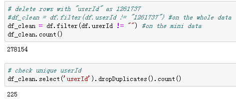
If we see closer at the “userId”, whose “firstName” was missing, we will find that those “userId” was actually empty strings (in the bid data was the user with the ID 1261737), with exactly 8346 records (with 778479 rows in the bid data), which I decided to treat as missing values and deleted. This might be someone who has only visited the Sparkify website without registering.

如果我們更靠近“ userId”(缺少“ firstName”)，我們會發現這些“ userId”實際上是空字符串(在出價數據中是ID為1261737的用戶)，正好有8346條記錄(778778)出價數據中的所有行)，我決定將其視為缺失值并刪除。 這可能是只訪問了Sparkify網站但未注冊的人。

After deleting the “problematic” userId, there was 255 unique users left (this number was 22277 for the big data).

刪除“有問題的”用戶ID后，剩下255個唯一用戶(大數據該數字為22277)。

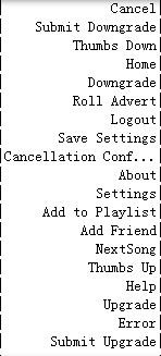
Let’s dig further on remaining missing values. As the data is event data, which means every operation of single users was recorded. I hypothesized that those missing values in the “artist” column might have an association with the certain actions (page visited) of the users, that’s why I check the visited “pages” associated with the missing “artist” and compared with the “pages” in the complete data and found that: “missing artist” is combined with all the other pages except “next song”, which means the “artist” (singer of the song) information is recorded only when a user hit “next song”.

讓我們進一步研究剩余的缺失值。 由于數據是事件數據，因此意味著記錄了單個用戶的每項操作。 我假設“藝術家”列中的那些缺失值可能與用戶的某些操作(訪問的頁面)相關聯，這就是為什么我檢查與缺失的“藝術家”相關聯的訪問過的“頁面”并與“頁面”進行比較的原因”中的完整數據，發現：“缺少歌手”與除“下一首歌”以外的所有其他頁面組合在一起，這意味著僅當用戶按下“下一首歌”時，“歌手”(歌曲的歌手)信息才會被記錄。

If I delete those “null” artist rows, there will be no missing values anymore in the data set and unique users number in the clean data set will still be 255.

如果刪除這些“空”藝術家行，則數據集中將不再缺少任何值，并且干凈數據集中的唯一用戶數仍為255。

After dealing with missing values, I transformed timestamp into epoch date, and simplified two categorical columns, extracting only “states” information from the “location” column and platform used by the users (marked as “agent”) from the “userAgent” column.

處理完缺失值后，我將時間戳轉換為時代日期，并簡化了兩個分類列，僅從“位置”列和“ userAgent”列中用戶使用的平臺(標記為“代理”)中提取“狀態”信息。

The data cleaning step is completed so far, and let’s start to explore the data and find out more information. As the final purpose is to predict churn, we need to first label the churned users (downgrade was also labeled in the same method). I used the “Cancellation Confirmation” events to define churn: those churned users who visited the “Cancellation Confirmation” page was marked as “1”, and who did not was marked as “0”. Similarly who visited page “Downgrade” at least once was marked as “1”, and who did not was marked as “0”. Now the data set with 278154 rows and columns shown below is ready for some exploratory analysis. Let’s do some comparisons between churned and stayed users.

到目前為止，數據清理步驟已經完成，讓我們開始探索數據并查找更多信息。 由于最終目的是預測用戶流失，因此我們需要先標記流失的用戶(降級也用相同的方法標記)。 我使用“取消確認”事件來定義用戶流失：那些訪問“取消確認”頁面的攪動用戶被標記為“ 1”，而沒有被標記為“ 0”的用戶。 同樣，至少訪問過一次“降級”頁面的人被標記為“ 1”，而沒有訪問過的人被標記為“ 0”。 現在，下面顯示的具有278154行和列的數據集已準備好進行一些探索性分析。 讓我們在流失用戶和停留用戶之間進行一些比較。

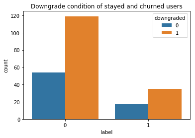
攪動和停留用戶的數量，性別，級別和降級情況 (Number, gender, level, and downgrade condition of churned and stayed users)

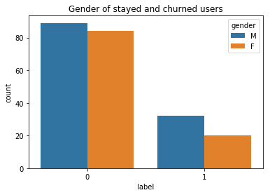
There were 52 churned and 173 stayed users in the small data set (those numbers were 5003 and 17274 respectively for the big data), with slightly more males than females in both groups (left figure below). It seemed that among the stayed users there were more people who have downgraded their account at least once (right figure below).

在小型數據集中，有52位攪拌用戶和173位常住用戶(大數據分別為5003和17274)，兩組中男性均比女性略多(下圖)。 似乎，在留下來的用戶中，有更多人至少一次降級了他們的帳戶(下圖右圖)。

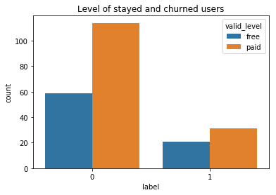
The “level” column has two values “free” and “paid”. Some users might have changed their level more than once. To check how “level” has differed between churned and stayed users, a “valid_level” column was created to record the latest level of users. As shown in the figure below, there are more paid users among the stayed users.

“級別”列具有兩個值“免費”和“已付費”。 一些用戶可能已多次更改其級別。 為了檢查攪動和停留的用戶之間的“級別”有何不同，創建了一個“ valid_level”列來記錄最新的用戶級別。 如下圖所示，在停留的用戶中有更多的付費用戶。

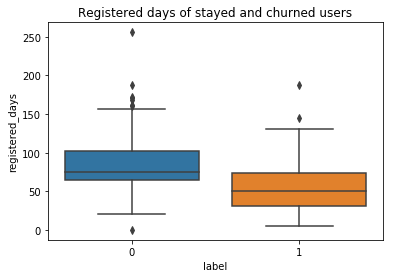
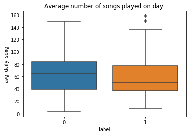
注冊天數，每天的歌曲數和每個會話的歌曲數 (Registered days, number of songs per day and number of songs per session)

The stayed users registered for more days than the churned users apparently, and the stayed users played on average more songs than the churned users both on a daily and a session base.

停留的用戶注冊的時間顯然比攪拌的用戶多，并且停留的用戶在每天和會話基礎上播放的歌曲平均比攪拌的用戶多。

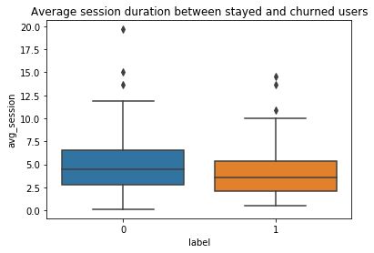
每日平均每次會話項目和平均會話持續時間 (Daily average item per session and average session duration)

As shown below, the daily average item per session was slightly higher for stayed users than churned users.

如下所示，對于留用用戶，每個會話的每日平均項目要略高于攪動用戶。

The average session duration was also longer for stayed users than churned users.

停留的用戶的平均會話持續時間也比攪動的用戶更長。

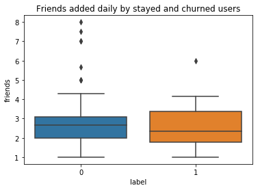
用戶活動分析 (User activities analysis)

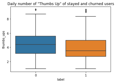
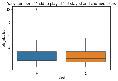
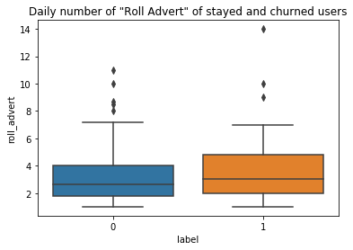
To analyze how the user activities differ between churned and stayed users, the daily average numbers of “thumbs up”, “add to playlist”, “add friend”, “roll adverts”, and” thumbs down” for each user were calculated. Those features were selected because they were the most visited pages among others (see table below).

為了分析攪動和停留用戶之間的用戶活動差異，計算了每個用戶每天的“豎起大拇指”，“添加到播放列表”，“添加朋友”，“滾動廣告”和“豎起大拇指”的平均數量。 選擇這些功能是因為它們是其他頁面中訪問量最大的頁面(請參見下表)。

As a result, churned users added fewer friends, gave less “thumbs up”, and added fewer songs into their playlists on a daily base than stayed users. While the churned users gave more “thumbs down” and rolled over more advertisements daily than stayed users.

結果，與留宿用戶相比，每天攪動的用戶添加更少的朋友，減少“豎起大拇指”，并且將更少的歌曲添加到他們的播放列表中。 盡管流失的用戶每天比停留的用戶更多地“豎起大拇指”，并滾動更多的廣告。

兩組用戶的平臺和位置 (The platform and location of two groups of users)

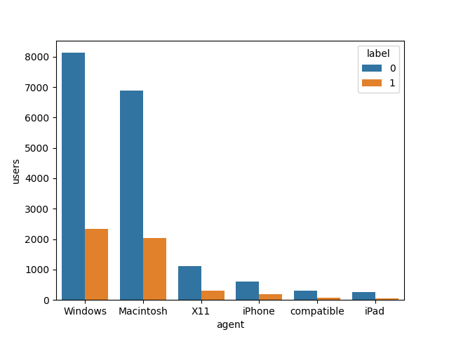
The platform (marked as “agent” in the table) used by users are plotted below. It appeared that the churning rates were different among the six agents. It means the platform on which the users are using Sparkify’s service might influence churn.

用戶繪制的平臺(表中標記為“代理”)如下圖所示。 看來這六個代理商的流失率是不同的。 這意味著用戶使用Sparkify服務的平臺可能會影響用戶流失。

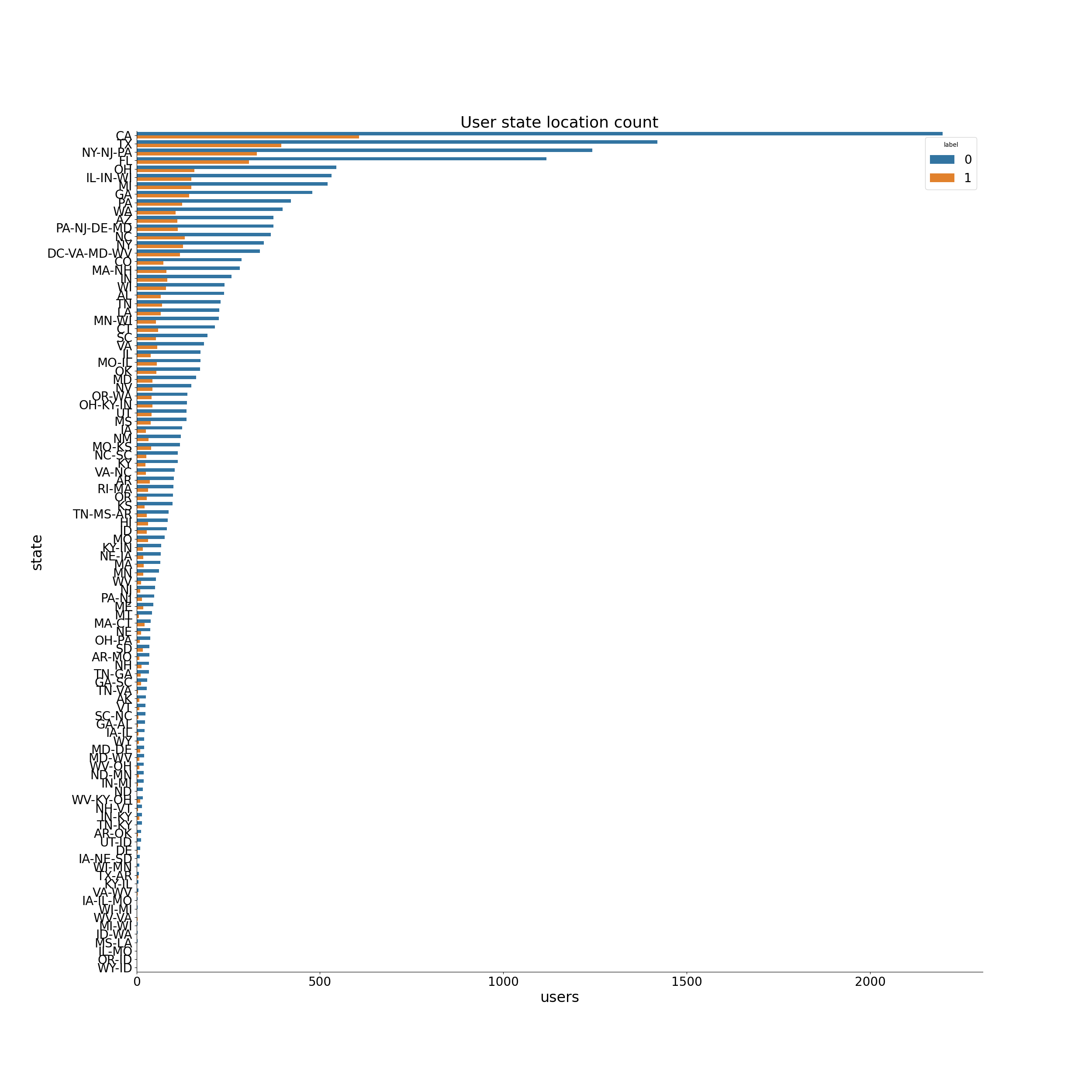
Similarly, the churning rates seemed to be changing in different states (see figure below).

同樣，不同國家的流失率似乎也在變化(見下圖)。

特征工程 (Feature engineering)

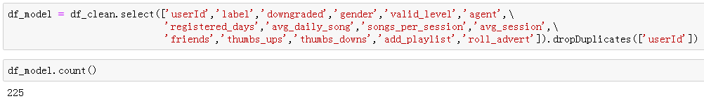
Before fitting any model, the following columns were assembled to create the final data set df_model for modeling.

在擬合任何模型之前，將以下各列進行組裝，以創建用于建模的最終數據集df_model 。

Response variable

響應變量

label: 1 for churned and 0 for not

標簽：1表示攪動，0表示不攪動

Explanatory variables (categorical)

解釋變量(分類)

downgraded: 1 for downgraded and 0 for not

降級：1表示降級，0表示??不降級

gender: M for male and F for female

性別：男為男，女為男

valid_level: free or paid

valid_level：免費或付費

agent: platform used by users with five categories (windows, macintosh, iPhone, iPad, and compatible)

代理：供五類用戶使用的平臺(Windows，macintosh，iPhone，iPad和兼容)

Explanatory variables (numeric)

解釋變量(數字)

registered_days: counted by the maximum value of “ts” (timestamp of actions) subtracted by “registration” timestamp and transformed to days

registered_days：以“ ts”(動作時間戳記)的最大值減去“ registration”時間戳記后轉換為天數

avg_daily_song: average song listened on a daily base

avg_daily_song：每天平均聽一首歌

songs_per_session: average songs listened per session

songs_per_session：每個會話平均聽過的歌曲

avg_session: average session duration

avg_session：平均會話持續時間

friends: daily number of friends added by a user

朋友：用戶每天添加的朋友數

thumbs up: daily number of thumbs up given by a user

豎起大拇指：用戶每天給出的豎起大拇指的次數

thumbs down: daily number of thumbs down given by a user

大拇指朝下：用戶每天給予的大拇指朝下的次數

add_playlist: daily number of “add to playlist” action

add_playlist：“添加到播放列表”操作的每日次數

roll_advert: daily number of “roll advert” action

roll_advert：“滾動廣告”操作的每日次數

Categorical variables ‘gender’,’valid_level’, and ’agent’ were first transformed into indexes using the StringIndexer.

首先使用StringIndexer將分類變量“ gender”，“ valid_level”和“ agent”轉換為索引。

# creating indexs for the categorical columns
indexers = [StringIndexer(inputCol=column, outputCol=column+"_index").fit(df_model) for column in ['gender','valid_level','agent'] ]pipeline = Pipeline(stages=indexers)
df_r = pipeline.fit(df_model).transform(df_model)
df_model = df_r.drop('gender','valid_level','agent')

And the numeric variables were first assembled into a vector using VectorAssembler and then scaled using StandardScaler.

然后，首先使用VectorAssembler將數字變量組裝為向量，然后使用StandardScaler對其進行縮放。

# assembeling numeric features to create a vector
cols=['registered_days','friends','thumbs_ups','thumbs_downs','add_playlist','roll_advert',\
      'daily_song','session_song','session_duration']assembler = VectorAssembler(inputCols=cols,outputCol="features")# use the transform method to transform df
df_model = assembler.transform(df_model)# standardize numeric feature vector
standardscaler=StandardScaler().setInputCol("features").setOutputCol("Scaled_features")
df_model = standardscaler.fit(df_model).transform(df_model)

In the end, all the categorical and numeric features were combined and again transformed into a vector.

最后，將所有類別和數字特征組合在一起，然后再次轉換為向量。

cols=['Scaled_features','downgraded','gender_index','valid_level_index','agent_index']
assembler = VectorAssembler(inputCols=cols,outputCol='exp_features')# use the transform method to transform df
df_model = assembler.transform(df_model)

造型 (Modeling)

As the goal was to predict a binary result (1 for churn and 0 for not), logistic regression, random forest, and gradient boosted tree classifiers were selected to fit the data set. F1 score and AUC were calculated as evaluation metrics. Because our training data was imbalanced (there were fewer churned than stayed users). And from the perspective of the company, incorrectly identifying a user who was going to churn is more costly. In this case, F1-score is a better metric than accuracy, because it provides a better measure of the incorrectly classified cases (for more information click here). AUC, on the other hand, gives us a perspective over how good the model is regarding the separability, in another word, distinguishing 1 (churn) from 0 (stay).

由于目標是預測二進制結果(流失為1，否則為0)，因此選擇了邏輯回歸，隨機森林和梯度增強樹分類器以適合數據集。 計算F1分數和AUC作為評估指標。 因為我們的訓練數據不平衡(攪動的人數少于留守的使用者)。 而且從公司的角度來看，錯誤地標識將要流失的用戶的成本更高。 在這種情況下，F1評分比準確度更好，因為它可以更好地衡量分類錯誤的案例(有關更多信息，請單擊此處 )。 另一方面， AUC為我們提供了關于模型關于可分離性的良好程度的觀點，換句話說，將1(攪動)與0(保持)區分開。

The data set was first broke into 80% of training data and 20% as a test set.

首先將數據集分為訓練數據的80％和測試集的20％。

rest, validation = df_model.randomSplit([0.8, 0.2], seed=42)

邏輯回歸模型 (Logistic regression model)

There were more stayed users than churned users in the whole data set, and in our training set the number of churned is 42, which represents only around 22% of total users. To solve this imbalance problem and get better prediction results, class_weights values were introduced into the model.

在整個數據集中，停留的用戶多于攪動的用戶，在我們的訓練集中，攪動的數量為42，僅占總用戶的22％。 為了解決此不平衡問題并獲得更好的預測結果，將class_weights值引入模型。

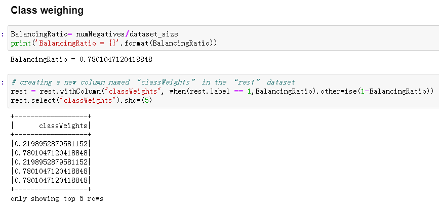
A logistic regression model with weighed features was built like the following and BinaryClassificationEvaluator was used to evaluate the model.

建立具有權重特征的邏輯回歸模型，如下所示，并使用BinaryClassificationEvaluator評估模型。

# Initialize logistic regression object
lr = LogisticRegression(labelCol="label", featuresCol="exp_features",weightCol="classWeights",maxIter=10)# fit the model on training set
model = lr.fit(rest)# Score the training and testing dataset using fitted model for evaluation purposes
predict_rest = model.transform(rest)
predict_val = model.transform(validation)# Evaluating the LR model using BinaryClassificationEvaluator
evaluator = BinaryClassificationEvaluator(rawPredictionCol="rawPrediction",labelCol="label")#F1 score
f1_score_evaluator = MulticlassClassificationEvaluator(metricName='f1')
f1_score_rest = f1_score_evaluator.evaluate(predict_rest.select(col('label'), col('prediction')))
f1_score_val = f1_score_evaluator.evaluate(predict_val.select(col('label'), col('prediction')))#AUC 
auc_evaluator = BinaryClassificationEvaluator()
roc_value_rest = auc_evaluator.evaluate(predict_rest, {auc_evaluator.metricName: "areaUnderROC"})
roc_value_val = auc_evaluator.evaluate(predict_val, {auc_evaluator.metricName: "areaUnderROC"})

The scores of the logistic regression model were like the following:

邏輯回歸模型的得分如下：

The F1 score on the train set is 74.38%
The F1 score on the test set is 73.10%
The areaUnderROC on the train set is 79.43%
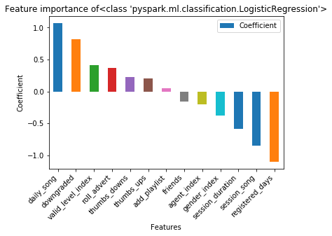
The areaUnderROC on the test set is 76.25%

And the feature importance is shown as the following. The feature registered days, the average number of songs listened per session, and the average session duration was negatively associated with churn, while the average number of songs listened per session and the action of downgraded was positively associated with churn. In another word, users who listen to more songs per day and downgraded at least once are more likely to churn. Whereas, the longer one session lasts and the more songs one listens per session, the less likely for this user to churn.

并且功能重要性如下所示。 該功能注冊的天數，每個會話中平均聽的歌曲數，平均會話持續時間與客戶流失率呈負相關，而每個會話中平均聽的歌曲數和降級行為與客戶流失率呈正相關。 換句話說，每天聽更多歌曲并且至少降級一次的用戶更有可能流失。 而一個會話持續的時間越長，每個會話聆聽的歌曲越多，則該用戶流失的可能性就越小。

It sounds a bit irrational that, the more songs one listens per day, the more likely for him to churn. To draw a safe conclusion, I would include more samples to fit the model again. This will be the future work.

聽起來有點不合理，因為每天聽的歌曲越多，他流失的可能性就越大。 為了得出一個安全的結論，我將包括更多樣本以再次適合模型。 這將是未來的工作。

隨機森林模型 (Random forest model)

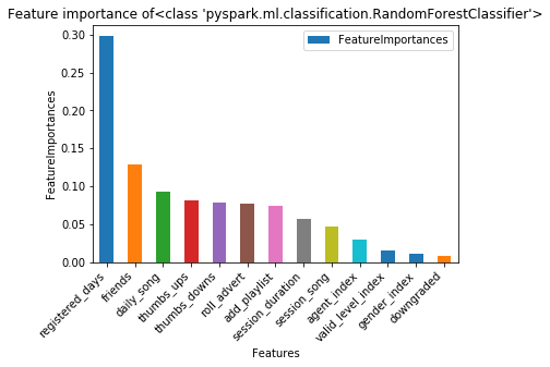
In a similar manner, a random forest model was fit into the training data, refer the original code here. And the metrics were as the following:

以類似的方式，將隨機森林模型擬合到訓練數據中，請在此處參考原始代碼。 指標如下：

The F1 score on the train set is 90.21%
The F1 score on the test set is 70.31%
The areaUnderROC on the train set is 98.21%
The areaUnderROC on the test set is 80.00%

There is obviously an overfitting problem. Both the F1 and AUC scores were very high for the training set and poorer in the test set. The feature importance analysis showed: Besides registered days and songs listened per day, the number of friends added, thumbs up, and thumbs down given on a daily base were the most important features regarding churn prediction. As future work, I would fit this model again on the big data set to see if adding samples will solve the overfitting problem.

顯然存在過度擬合的問題。 F1和AUC分數在訓練集中都非常高，而在測試集中則較差。 特征重要性分析表明：除了記錄的天數和每天聽的歌曲之外，每天增加的好友數，豎起大拇指和豎起大拇指都是關于流失預測的最重要特征。 在以后的工作中，我將再次將該模型適合大數據集，以查看添加樣本是否可以解決過擬合問題。

梯度提升樹模型 (Gradient boosted tree model)

GBT model showed a more severe overfitting problem. A suggestion for improvement will be the same as mentioned before. Try on the big data set first, if necessary do finer feature engineering or try other methods.

GBT模型顯示了更嚴重的過度擬合問題。 改進的建議與前面提到的相同。 首先嘗試大數據集，必要時進行更精細的功能設計或嘗試其他方法 。

The F1 score on the train set is 99.47%
The F1 score on the test set is 68.04%
The areaUnderROC on the train set is 100.00%
The areaUnderROC on the test set is 64.58%

超參數調整和交叉驗證 (Hyperparameter tuning and cross-validation)

According to the F1 and AUC scores of all three models, I decided to pick the logistic regression model to do further hyperparameter tuning and 3-fold cross-validation.

根據這三個模型的F1和AUC分數，我決定選擇邏輯回歸模型進行進一步的超參數調整和3倍交叉驗證。

# logistic regression model parameters tuning
lrparamGrid = ParamGridBuilder() \
    .addGrid(lr.elasticNetParam,[0.0, 0.1, 0.5]) \
    .addGrid(lr.regParam,[0.0, 0.05, 0.1]) \
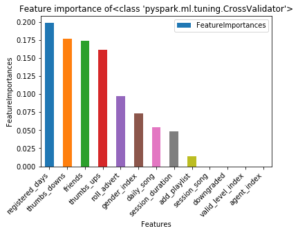
    .build()

However, except for an obvious improvement in model performance on the training set. Both the F1 and AUC scores were lower on the test set. For an overfitting situation, parameter tuning was a bit tricky, and cross-validation did not help in this case to improve model performance, check the link here which might through some insight into this problem.

但是，除了訓練集上的模型性能有明顯改善外。 F1和AUC分數在測試集上均較低。 對于過度擬合的情況，參數調整有些棘手，在這種情況下，交叉驗證無助于提高模型性能，請查看此處的鏈接 ，這可能會通過一些洞察力來解決此問題。

The F1 score on the train set is 87.73%
The F1 score on the test set is 72.74%
The areaUnderROC on the train set is 91.27%
The areaUnderROC on the test set is 78.33%

Feature importance of logistic regression after parameter tuning and cross-validation showed a different pattern from before. The registered day was the most promising indicator of churn (this information might with little interest to the service provider company). Besides, the number of thumbs-ups, friends added, thumbs-downs and roll advert were the features with the highest importance.

參數調整和交叉驗證后邏輯回歸的特征重要性顯示出與以前不同的模式。 注冊日是流失率最有希望的指標(服務提供商公司可能對此信息不太感興趣)。 此外，最重要的功能是大拇指向上，朋友添加，大拇指向下和滾動廣告的數量。

結論 (Conclusion)

In this project, churn prediction was performed based on an event data set for a music streaming provider. This was basically a binary classification problem. After loading and cleaning data, I performed some exploratory analysis and provided insights on the next step of feature engineering. All together 13 explanatory features were selected and logistic regression, random forest, and gradient-boosted tree models were fitted respectively to a training data set.

在該項目中，根據針對音樂流媒體提供商的事件數據集執行了流失預測。 這基本上是一個二進制分類問題。 加載和清理數據后，我進行了一些探索性分析，并就功能設計的下一步提供了見解。 總共選擇了13個解釋特征，并將邏輯回歸，隨機森林和梯度提升樹模型分別擬合到訓練數據集。

The model performance was the best for the logistic regression on small data set, with an F1 score of 73.10 on the test set. The other two models were both suffered from overfitting. Hyperparameter tuning and cross-validation was not very helpful in solving overfitting, probably because of a small number of sample size. Due to time and budget limitations, the final models were not tested on the big data set. However, the completely scalable process shed a light on solving the churn prediction problem on big data with Spark on Cloud.

模型性能對于小數據集的邏輯回歸最好，測試集的F1得分為73.10。 另外兩個模型都過度擬合。 超參數調整和交叉驗證對解決過度擬合的幫助不是很大，這可能是因為樣本數量很少。 由于時間和預算的限制，最終模型未在大數據集上進行測試。 但是，完全可擴展的過程為使用Spark on Cloud解決大數據的客戶流失預測問題提供了啟示。

討論區 (Discussion)

Feature engineering

特征工程

How to chose the proper explanatory features was one of the most critical steps in this task. After EDA, I simply included all the features that I created. I wanted to create more features, however, the further computation was dragged down by limited computation capacity. There are some techniques ( for example the ChiSqSelector provided by Spark ML) on feature engineering that might help in this step. The “state” column had 58 different values (100 for the big data). I tried to turn them into index values using StringIndexer and include it to the explanatory feature. However, it was not possible to build a random forest/GBTs model with indexes exceeded the maxBins (= 32), that’s why I had to exclude this feature. If it was possible to use the dummy variable of this feature, the problem could have been avoided. It was a pity that I run out of time and did not manage to do a further experiment.

如何選擇適當的解釋功能是此任務中最關鍵的步驟之一。 在EDA之后，我只包含了我創建的所有功能。 我想創建更多功能，但是，由于計算能力有限，進一步的計算被拖累了。 在要素工程上有一些技術 (例如，Spark ML提供的ChiSqSelector)可能在此步驟中有所幫助。 “狀態”列具有58個不同的值(大數據為100個)。 我嘗試使用StringIndexer將它們轉換為索引值，并將其包含在說明功能中。 但是，無法建立索引超過maxBins(= 32)的隨機森林/ GBTs模型，這就是為什么我必須排除此功能。 如果可以使用此功能的啞變量，則可以避免該問題。 遺憾的是我時間不夠用，沒有做進一步的實驗。

Computing capacity

計算能力

Most of the time I spent on this project was “waiting” for the result. It was very frustrating that I had to stop and run the codes from the beginning over and over again due to stage errors because the cluster was running out of memory. To solve this problem, I had to separate my code into two parts (one for modeling) and the other for plotting and run them separately. And I have to reduce the number of explanatory variables that I created. It was a pity that I only managed once to run the simple version of code for the big data set on AWS cluster (refer to the code here) and had to stop because it took too much time and cost. The scores of the build models on the big data set were unfortunately not satisfying. However, the last version of codes (Sparkify_visualization and Sparkify_modeling in Github repo) should be completely scalable. The performance of models on big data set should be improved if the latest codes are to be run on the big data again.

我在這個項目上花費的大部分時間都是在“等待”結果。 令人沮喪的是，由于階段錯誤，我不得不從頭開始一遍又一遍地停止并運行代碼，因為群集內存不足。 為了解決這個問題，我不得不將代碼分成兩部分(一個用于建模)，另一個用于繪圖并分別運行。 而且我必須減少創建的解釋變量的數量。 遺憾的是，我只為AWS集群上的大數據集運行了簡單版本的代碼(請參閱此處的代碼)，卻不得不停止，因為這花費了太多時間和成本。 不幸的是，大數據集上構建模型的分數并不令人滿意。 但是，代碼的最新版本(Github存儲庫中的Sparkify_visualization和Sparkify_modeling)應該是完全可伸縮的。 如果要在大數據上再次運行最新代碼，則應提高大數據集上模型的性能。

Testing selective sampling method

測試選擇性抽樣方法

Because the training data set is imbalanced with more “0” labeled rows than “1”, I wanted to try if randomly selecting the same number of “0” rows as “1” rows would have improved the model performance. Due to the time limit, it will be only the work for the future.

因為訓練數據集的“ 0”行比“ 1”行更多，所以我想嘗試一下，如果隨機選擇與“ 1”行相同數量的“ 0”行可以改善模型性能。 由于時間限制，這只是未來的工作。

ps: one extra tip which might be very useful, perform “cache” on critical points to speed up the program.

ps：一個可能非常有用的額外技巧，對關鍵點執行“緩存”以加快程序運行速度。

Any discussion is welcome! Please reach me through LinkedIn and Github

歡迎任何討論！ 請通過LinkedIn和Github與我聯系