· 1. Introduction· 2. Exploratory Data Analysis ° 2.1 Pattern Changes ° 2.2 Correlation Between Features· 3. Anomaly Detection and Pattern Recognition ° 3.1 Point Anomaly Detection (System Fault) ° 3.2 Collective Anomaly Detection (External Event) ° 3.3 Clustering and Pattern Recognition (External Event)· 4. Conclusion·

· 1.簡介 · 2.探索性數據分析 °2.1 模式更改 °2.2 特征之間的相關性 · 3.異常檢測和模式識別 °3.1 點異常檢測(系統故障) °3.2 集體異常檢測(外部事件) °3.3 聚類和模式認可(外部事件) · 4.結論 ·

Note: The detailed project report and the datasets used in this post can be found in my GitHub Page.

注意 ：本文中使用的詳細項目報告和數據集可以在我的GitHub Page中找到。

1.簡介 (1. Introduction)

This project was assigned to me by a client. There is no non-disclosure agreement required and the project does not contain any sensitive information. So, I decide to make this project public as part of my personal data science portfolio while anonymizing the client’s information.

該項目是由客戶分配給我的。 不需要保密協議，該項目不包含任何敏感信息。 因此，我決定將該項目公開，作為我的個人數據科學投資組合的一部分，同時匿名化客戶的信息。

In the project, there are two data sets, each consists of one week of sensor readings are provided to accomplish the following four tasks:

在該項目中，有兩個數據集，每個數據集包含一個星期的傳感器讀數，以完成以下四個任務：

1. Find anomalies in the data set to automatically flag events

1.在數據集中查找異常以自動標記事件

2. Categorize anomalies as “System fault” or “external event”

2.將異常分類為“系統故障”或“外部事件”

3. Provide any other useful conclusions from the pattern in the data set

3.根據數據集中的模式提供其他有用的結論

4. Visualize inter-dependencies of the features in the dataset

4.可視化數據集中要素的相互依賴性

In this report I am going to briefly walk through the steps I use for data analysis, visualization of feature correlation, machine learning techniques to automatically flag “system faults” and “external events” and my findings from the data.

在本報告中，我將簡要介紹我用于數據分析，特征關聯可視化，機器學習技術以自動標記“系統故障”和“外部事件”以及我從數據中發現的步驟。

2.探索性數據分析 (2. Exploratory Data Analysis)

My code and results in this section can be found here.

我在本節中的代碼和結果可以在這里找到。

The dataset comes with two CSV files, both of which can be accessed from my GitHub Page. I first import and concatenate them into one Pandas dataframe in Python. Some rearrangements are made to remove columns except the 11 features that we are interested in:

該數據集帶有兩個CSV文件，都可以從我的GitHub Page中訪問它們。 我首先將它們導入并用Python連接到一個Pandas數據框中。 除我們感興趣的11個功能外，還進行了一些重新排列以刪除列：

• Ozone
  臭氧
• Hydrogen Sulfide
  硫化氫
• Total VOCs
  總VOC
• Carbon Dioxide
  二氧化碳
• PM 1
  1號紙
• PM 2.5
  下午2.5
• PM 10
  下午10點
• Temperature (Internal & External)
  溫度(內部和外部)
• Humidity (Internal & External).
  濕度(內部和外部)。

The timestamps span from May 26 to June 9, 2020 (14 whole days in total) in EDT (GMT-4) time zone. By subtraction, different intervals are found between each reading, ranging from 7 seconds to 3552 seconds. The top 5 frequent time intervals are listed below in Table 1, where most of them are close to 59 and 60 seconds, so it can be concluded that the sensor reads every minute. However, the inconsistency of reading intervals might be worth looking into if it is no deliberate interference involved since it might cause trouble in future time series analysis.

時間戳跨越EDT(GMT-4)時區的2020年5月26日至6月9日(共14天)。 通過減法，可以在每個讀數之間找到不同的間隔，范圍從7秒到3552秒。 下面的表1中列出了前5個最頻繁的時間間隔，其中大多數時間間隔接近59秒和60秒，因此可以得出結論，傳感器每分鐘都會讀取一次。 但是，如果不涉及故意的干擾，則可能需要研究讀取間隔的不一致，因為這可能會在以后的時間序列分析中造成麻煩。

For each of the features, the time series data are on different scales, so they are normalized in order for better visualization and machine learning efficiencies. Then they are plotted and visually inspected to discover any interesting patterns.

對于每個功能，時間序列數據的比例不同，因此對其進行了歸一化，以實現更好的可視化和機器學習效率。 然后將它們繪制出來并進行視覺檢查，以發現任何有趣的圖案。

2.1模式變更 (2.1 Pattern Changes)

Some of the features seem to share similar pattern changes at specific time points. Three of the most significant ones (Temperature External, Humidity External, and Ozone) are shown below in Figure 1. It can be clearly seen that the areas highlighted with pink tend to have flat signals while the unhighlighted areas are sinusoidal.

一些功能似乎在特定時間點共享相似的模式更改。 圖1中顯示了三個最重要的區域(外部溫度，外部濕度和臭氧)。可以清楚地看到，用粉紅色突出顯示的區域傾向于發出平坦的信號，而未突出顯示的區域則是正弦的。

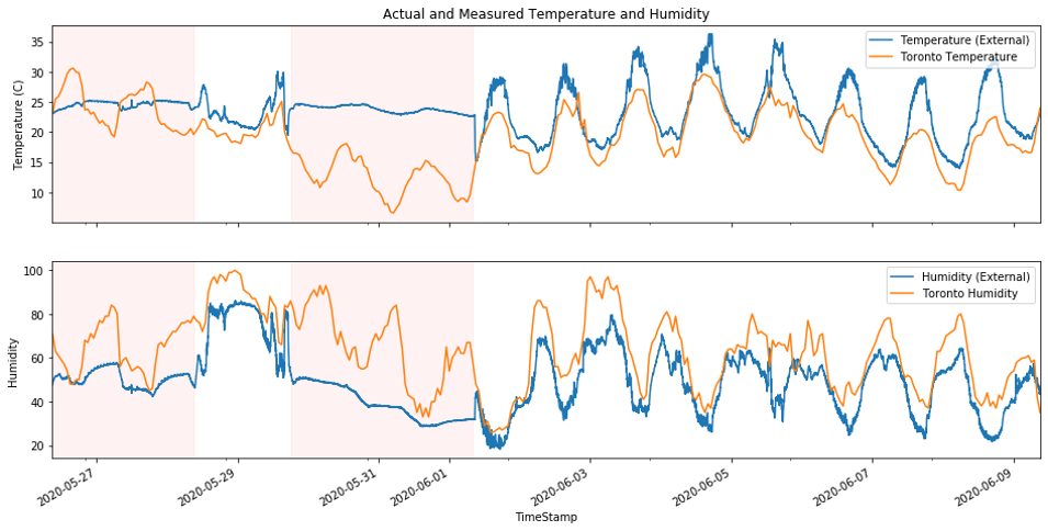
According to common sense, the outdoor temperature reaches its high point at noon and goes down at night, I start to wonder the possibility that different test environments were involved during this 14-day period. To test the idea, Toronto weather data is queried from Canada Weather Stats [1]. The temperature and relative humidity are overlaid and compared with the external temperature and humidity in this dataset. The plot is shown in Figure 2. It can be seen that the actual temperature and humidity fluctuate in a sinusoidal fashion. Most parts of the temperature and humidity readings correlate well with the weather data, while the areas highlighted in pink remains relatively invariant. I am not provided with any relevant information on the environments that the measurements were taken, but from the plot, it can be reasonably inferred that the device has been relocated between indoor and outdoor environments during the 14-day period. This is also tested later in the automatic anomaly detection in Section 3.3.

根據常識，室外溫度會在中午達到最高點，并在晚上下降，我開始懷疑在這14天的時間內是否涉及不同的測試環境。 為了驗證這個想法，可以從加拿大天氣統計中查詢多倫多的天氣數據[1]。 覆蓋溫度和相對濕度，并與該數據集中的外部溫度和濕度進行比較。 該圖如圖2所示。可以看出，實際溫度和濕度以正弦形式波動。 溫度和濕度讀數的大部分與天氣數據具有良好的相關性，而用粉紅色突出顯示的區域則相對不變。 在進行測量的環境中，我沒有得到任何相關信息，但是從繪圖中可以合理地推斷出該設備在14天的時間內已在室內和室外環境之間重新放置。 稍后還將在3.3節中的自動異常檢測中對此進行測試。

2.2特征之間的關聯 (2.2 Correlation Between Features)

Correlation is a technique for investigating the relationship between two quantitative, continuous variables in order to represent their inter-dependencies. Among different correlation techniques, Pearson’s correlation is the most common one, which measures the strength of association between the two variables. Its correlation coefficient scales from -1 to 1, where 1 represents the strongest positive correlation, -1 represents the strongest negative correlation and 0 represents no correlation. The correlation coefficients between each pair of the dataset are calculated and plotted as a heatmap, shown in Table 2. The scatter matrix of selected features is also plotted and attached in the Appendix section.

關聯是一種技術，用于研究兩個定??量的連續變量之間的關系，以表示它們之間的相互依賴性。 在不同的相關技術中，Pearson相關是最常見的一種，它測量兩個變量之間的關聯強度。 其相關系數從-1到1，其中1表示最強的正相關，-1表示最強的負相關，0表示無相關。 計算每對數據集之間的相關系數，并將其繪制為熱圖，如表2所示。選定要素的散布矩陣也被繪制并附在附錄部分。

The first thing to be noticed is that PM 1, PM 2.5, and PM 10 are highly correlated with each other, which means they always fluctuate in the same fashion. Ozone is negatively correlated with Carbon Dioxide and positively correlates with Temperature (Internal) and Temperature (External). On the other hand, it is surprising not to find any significant correlation between Temperature (Internal) and Temperature (External), possibly due to the superior thermal insulation of the instrument. However, since there is no relevant knowledge provided, no conclusions can be made on the reasonability of this finding. Except for Ozone, Temperature (Internal) is also negatively correlated with Carbon Dioxide, Hydrogen Sulfide, and the three particulate matter measures. On the contrary, Temperature (External) positively correlates with Humidity (Internal) and three particulate matter measures, while negatively correlates with Humidity (External), just as what can be found from the time series plots in Figure 1.

首先要注意的是，PM 1，PM 2.5和PM 10彼此高度相關，這意味著它們始終以相同的方式波動。 臭氧與二氧化碳呈負相關，與溫度(內部)和溫度(外部)呈正相關。 另一方面，令人驚訝的是，沒有發現溫度(內部)和溫度(外部)之間的任何顯著相關性，這可能是由于儀器具有出色的隔熱性。 但是，由于沒有提供相關的知識，因此無法就此發現的合理性得出任何結論。 除臭氧外，溫度(內部)還與二氧化碳，硫化氫和三種顆粒物度量值呈負相關。 相反，溫度(外部)與濕度(內部)和三個顆粒物度量呈正相關，而與濕度(外部)呈負相關，正如圖1的時間序列圖所示。

3.異常檢測和模式識別 (3. Anomaly Detection and Pattern Recognition)

In this section, various anomaly detection methods are examined based on the dataset. The data come without labels, so there is no knowledge or classification rule is provided to distinguish between “system faults”, “external events” and others. Any details of the instrument and experiments are not provided either. Therefore, my results in this section might deviate from expectations, but I am trying my best to make assumptions, define problems, and then accomplish them based on my personal experience. The section consists of three parts: Point Anomaly Detection, Collective Anomaly Detection, and Clustering.

在本節中，將基于數據集檢查各種異常檢測方法。 數據沒有標簽，因此沒有提供知識或分類規則來區分“系統故障”，“外部事件”和其他。 也沒有提供儀器和實驗的任何細節。 因此，我在本節中的結果可能會偏離預期，但我會盡力做出假設，定義問題，然后根據我的個人經驗完成這些假設。 本節包括三個部分：點異常檢測，集體異常檢測和聚類。

3.1點異常檢測(系統故障) (3.1 Point Anomaly Detection (System Fault))

Point anomalies, or global outliers, are those data points that are entirely outside the scope of the usual signals without any support of close neighbors. It is usually caused by human or system error and needs to be removed during data cleaning for better performance in predictive modeling. In this dataset, by assuming the “system faults” are equivalent to such point anomalies, there are several features that are worth examining, such as the examples shown below in Figure 3.

點異常或全局離群值是完全不在常規信號范圍內而沒有任何近鄰支持的數據點。 它通常是由人為或系統錯誤引起的，需要在數據清理過程中將其刪除以在預測建模中獲得更好的性能。 在此數據集中，通過假設“系統故障”等效于此類點異常，有幾個特性值得研究，例如下面的圖3中所示的示例。

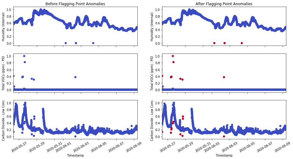
Here, from Humidity (Internal) to Total VOC to Carbon Dioxide, each represents a distinct complexity of point anomaly detection tasks. In the first one, three outliers sit on the level of 0, so a simple boolean filter can do its job of flagging these data points. In the second one, the outliers deviate significantly from the signal that we are interested in, so linear thresholds can be used to separate out the outliers. Both cases are easy to implement because they can be done by purely experience-based methods. When it comes to the third case, it is not possible to use a linear threshold to separate out the outliers since even if they deviate from its neighbors, the values may not be as great as the usual signals at other time points.

在這里，從濕度(內部)到總VOC到二氧化碳，每個都代表了點異常檢測任務的獨特復雜性。 在第一個中，三個離群值位于0級別上，因此一個簡單的布爾過濾器可以完成標記這些數據點的工作。 在第二個中，離群值明顯偏離了我們感興趣的信號，因此可以使用線性閾值來分離離群值。 兩種情況都易于實現，因為它們可以通過純粹基于經驗的方法來完成。 在第三種情況下，不可能使用線性閾值來分離離群值，因為即使離群值偏離其鄰域，其值也可能不如其他時間點的正常信號大。

For such cases, there are many ways to approach. One of the simple ways is to calculate the rolling mean or median at each time point and test if the actual value is within the prediction interval that is calculated by adding and subtracting a certain fluctuation range from the central line. Since we are dealing with outliers in our case, the rolling median is more robust, so it is used in this dataset.

對于這種情況，有很多方法可以解決。 一種簡單的方法是計算每個時間點的滾動平均值或中位數，并測試實際值是否在預測區間內，該預測區間是通過從中心線增加或減去某個波動范圍而得出的。 由于在這種情況下我們正在處理離群值，因此滾動中位數更為穩健，因此在此數據集中使用了滾動中位數。

From Figure 4, it is even clearer to demonstrate this approach: Equal-distance prediction intervals are set based on the rolling median. Here, the rolling window is set to 5, which means that for each data point, we take four of its closest neighbors and calculate the median as the center of prediction. Then a prediction interval of ±0.17 is padded around the center. Any points outside are considered as outliers.

從圖4中可以更清楚地證明這種方法：等距預測間隔基于滾動中值設置。 在這里，滾動窗口設置為5，這意味著對于每個數據點，我們取其四個最近的鄰居并計算中位數作為預測中心。 然后，在中心周圍填充±0.17的預測間隔。 外部的任何點均視為異常值。

It is straightforward and efficient to detect the point anomalies using this approach. However, it has deficiencies and may not be reliable enough to deal with more complex data. In this model, there are two parameters: rolling window size and prediction interval size, both of which are defined manually through experimentations with the given data. We are essentially solving the problem encountered when going from case 2 to case 3 as seen in Figure 3 by enabling the self-adjusting capability to the classification boundary between signal and outliers according to time. However, the bandwidth is fixed, so it becomes less useful in cases when the definition of point anomalies changes with time. For example, the definition of a super cheap flight ticket might be totally different between a normal weekday and the holiday season.

使用這種方法來檢測點異常非常簡單有效。 但是，它有缺陷并且可能不夠可靠，無法處理更復雜的數據。 在此模型中，有兩個參數：滾動窗口大小和預測間隔大小，這兩個參數都是通過對給定數據進行實驗來手動定義的。 如圖3所示，我們基本上是通過從情況2轉到情況3來解決問題，方法是根據時間啟用信號和離群值之間的分類邊界的自調整功能。 但是，帶寬是固定的，因此在點異常的定義隨時間變化的情況下，帶寬變得不再有用。 例如，在正常工作日和假日季節之間，超廉價機票的定義可能完全不同。

That is when machine learning comes into play, where the model can learn from the data to adjust the parameters by itself when the time changes. It will know when a data point can be classified as point anomaly or not at a specific time point. However, I cannot construct such a supervised machine learning model on this task for this dataset since the premise is to have labeled data, and ours is not. It would be still be suggested to go along this path in the future because with such a model, the most accurate results will be generated no matter how complex the system or the data are.

那就是機器學習開始發揮作用的時候，模型可以從數據中學習，以在時間變化時自行調整參數。 它將知道何時可以在特定時間點將數據點歸類為點異常或不將其分類為點異常。 但是，我不能為此數據集在此任務上構造這樣的監督機器學習模型，因為前提是要有標記數據，而我們沒有。 仍建議在將來沿這條路走，因為使用這種模型，無論系統或數據多么復雜，都將產生最準確的結果。

Even though supervised learning methods would not work in this task, there are unsupervised learning techniques that can be useful such as clustering, also discussed in subsection 3.3. Clustering can group unlabeled data by using similarity measures, such as the distance between data points in the vector space. Then the point anomalies can be distinguished by selecting those far away from cluster centers. However, in order to use clustering for point anomaly detection in this dataset, we have to follow the assumption that external events are defined with the scope of multiple features instead of treating every single time series separately. More details on this are discussed in the following two subsections 3.2 and 3.3.

即使在這種任務下不能使用監督學習方法，也有一些有用的無監督學習技術，例如聚類，也在3.3小節中進行了討論。 聚類可以使用相似性度量(例如向量空間中數據點之間的距離)對未標記的數據進行分組。 然后可以通過選擇遠離聚類中心的點來區分點異常。 但是，為了將聚類用于此數據集中的點異常檢測，我們必須遵循這樣的假設：外部事件是在多個特征的范圍內定義的，而不是分別處理每個時間序列。 以下兩個小節3.2和3.3討論了有關此問題的更多詳細信息。

3.2集體異常檢測(外部事件) (3.2 Collective Anomaly Detection (External Event))

If we define the “system fault” as point anomaly, then there are two directions to go with the “external event”. One of them is to define it as a collective anomaly that appears in every single time-series signals. The idea of collective anomaly is on the contrary to point anomaly. Point anomalies are discontinued values that are greatly deviated from usual signals while collective anomalies are usually continuous, but the values are out of expectations, such as significant increase or decrease at some time points. In this subsection, all 11 features are treated separately as a single time series. Then the task is to find the abrupt changes that happen in each of them.

如果我們將“系統故障”定義為點異常，則“外部事件”有兩個方向。 其中之一是將其定義為出現在每個時間序列信號中的集體異常。 集體異常的概念與點異常相反。 點異常是不連續的值，與通常的信號有很大的偏離，而集體異常通常是連續的，但是這些值超出了預期，例如在某些時間點顯著增加或減少。 在本小節中，所有11個功能部件均被視為一個時間序列。 然后的任務是找到每個變化都發生的突變。

For such a problem, one typical approach is to tweak the usage of time series forecasting: we can fit a model to a certain time period before and predict the value after. The actual value is then compared to see if it falls into the prediction interval. It is very similar to the rolling median method used in the previous subsection, but only the previous time points are used here instead of using neighbors from both directions.

對于這樣的問題，一種典型的方法是調整時間序列預測的用法：我們可以將模型擬合到之前的某個時間段，然后預測之后的值。 然后將實際值進行比較，以查看其是否落在預測間隔內。 它與上一小節中使用的滾動中值方法非常相似，但是此處僅使用前一個時間點，而不是使用雙向的鄰居。

There are different options for the model as well. Traditional time series forecast models like SARIMA is a good candidate, but the model may not be complex enough to accommodate the “patterns” that I mentioned in Section 2.1 and Section 3.3. Another option is to train a supervised regression model for the time series, which is quite widely used nowadays.

該模型也有不同的選擇。 傳統的時間序列預測模型(如SARIMA)是不錯的選擇，但該模型可能不夠復雜，無法適應我在2.1節和3.3節中提到的“模式”。 另一種選擇是為時間序列訓練監督回歸模型，該模型在當今已被廣泛使用。

The idea is simple: Features are extracted from the time series using the concept of the sliding window, as seen in Table 3 and Figure 5. The sliding window size (blue) is set to be the same as the desired feature number k. Then for each data point (orange) in the time series, the features are data point values from its lag 1 to lag k before. As a result, a time series with N samples is able to be transformed into a table of N-k observations and k features. Next, by implementing the concept of “forward chaining”, each point is predicted by the regression model trained using observations from indices of 0 to k-1. In addition to the main regression model, two more quantile regressors are trained with different significance levels to predict the upper and lower bounds of the prediction interval, with which we are able to tell the actual value is above or below the interval band.

這個想法很簡單：使用滑動窗口的概念從時間序列中提取特征，如表3和圖5所示。滑動窗口的大小(藍色)設置為與所需特征編號k相同。 然后，對于時間序列中的每個數據點(橙色)，特征都是從滯后1到滯后k的數據點值。 結果，具有N個樣本的時間序列可以轉換為Nk個觀測值和k個特征的表。 接下來，通過實施“正向鏈接”的概念，通過使用從0到k-1的索引的觀察值訓練的回歸模型來預測每個點。 除了主要的回歸模型外，還訓練了另外兩個具有不同顯著性水平的分位數回歸器，以預測預測區間的上限和下限，由此我們可以判斷出實際值是在區間帶之上還是之下。

This method is applied to the given dataset, and an example is shown below as a result in Figure 6. The Ozone time series is hourly sampled for faster training speed and the features are extracted and fed into three Gradient Boosting Regressor models (1 main and 2 quantile regressors) using Scikit-Learn. The significance levels are chosen so that the prediction level represents a 90% confidence interval (shown as green in Figure 6 Top). The actual values are then compared with the prediction interval and flagged with red (unexpected increase) and blue (unexpected decrease) in Figure 6 Bottom.

此方法適用于給定的數據集，結果如圖6所示。下面是示例。每小時對臭氧時間序列進行采樣，以提高訓練速度，并提取特征并將其輸入到三個Gradient Boosting Regressor模型(1個主要模型和2個分位數回歸)使用Scikit-Learn。 選擇顯著性水平，以便預測水平代表90％的置信區間(在圖6頂部顯示為綠色)。 然后，將實際值與預測間隔進行比較，并在圖6底部用紅色(意外增加)和藍色(意外減少)標記。

The results may not be super impressive yet, because more work still needs to be done around regression model selections and hyperparameter fine-tunings. However, it is already showing its capability of fagging these abrupt increases and decreases in all these spikes. One great thing about using machine learning models is that the model learns and evolves by itself when feeding with data. From Figure 6 Bottom, it can be seen that the last three hills (after about 240 hours) have fewer flagged points than the previous ones. It is not only because the magnitudes are smaller, but also due to the fact that the model is learning from the previous experience and start to adapt to the “idea” that it is now in “mountains” and periodic fluctuations should be expected. Therefore, it is not hard to conclude that the model performance can get better and better if more data instances are fed.

結果可能不會令人印象深刻，因為圍繞回歸模型選擇和超參數微調仍需要做更多的工作。 但是，它已經顯示出阻止所有這些尖峰中這些突然增加和減少的能力。 使用機器學習模型的一大好處是，模型在輸入數據時會自行學習和演化。 從圖6的底部可以看出，最后三個山丘(約240小時后)的標記點比以前的要少。 這不僅是因為幅度較小，而且還因為該模型是從以前的經驗中學到并開始適應“思想”的事實，因此它現在處于“山脈”中，應該預期會出現周期性波動。 因此，不難得出這樣的結論：如果饋送了更多的數據實例，則模型性能會越來越好。

Beyond this quantile regression model, deep learning models such as LSTM might be able to achieve better performance. Long Short Term Memory (LSTM) is a specialized artificial Recurrent Neural Network (RNN) that is one of the state-of-the-art choices of sequence modeling due to its special design of feedback connections. However, it takes much longer time and effort to set up and fine-tune the network architecture, which exceeds the time allowance of this project, so it is not included as the presentable content in this report.

除了這種分位數回歸模型之外，諸如LSTM之類的深度學習模型也許還能獲得更好的性能。 長短期記憶(LSTM)是一種專門的人工循環神經網絡(RNN)，由于其特殊的反饋連接設計，它是序列建模的最新選擇之一。 但是，建立和微調網絡體系結構需要花費更多的時間和精力，這超出了該項目的時間限制，因此在本報告中未將其包括在內。

Again, on the other hand, as I mentioned in previous sections, the provided data does not come with labels showing which data points are considered as anomalies. It does cause difficulties in the collective anomaly detection task discussed in this subsection by limiting the model choices and performance. In the future, if some labels are provided, it will become a semi-supervised or supervised learning problem, so that it will become easier to achieve better results.

同樣，另一方面，正如我在前面的部分中提到的那樣，所提供的數據沒有附帶標簽，這些標簽顯示哪些數據點被視為異常。 通過限制模型的選擇和性能，確實在本小節討論的集體異常檢測任務中造成了困難。 將來，如果提供一些標簽，它將成為半監督或有監督的學習問題，以便變得更容易獲得更好的結果。

3.3聚類和模式識別(外部事件) (3.3 Clustering and Pattern Recognition (External Event))

As I mentioned in subsection 3.2 above, recognizing the “external events” can be approached in two directions: one is to treat every time series separately and monitor any unexpected changes happened to the sensor signals, and the other one is to assume the events affect multiple features at the same time so that we hope to distinguish the events by looking at the unique characteristics shown in different features. In this case, if we have labeled data, it would be a common classification problem, but even without labels, we are still able to approach by clustering.

正如我在上面的3.2小節中提到的，認識“外部事件”可以從兩個方向進行：一個是分別處理每個時間序列并監視傳感器信號發生的任何意外變化，另一個是假設事件影響因此，我們希望通過查看不同功能中顯示的獨特特征來區分事件。 在這種情況下，如果我們為數據加標簽，這將是一個常見的分類問題，但是即使沒有標簽，我們仍然能夠通過聚類進行處理。

Clustering is an unsupervised machine learning technique that finds similarities between data according to the characteristics and groups similar data objects into clusters. It can be used as a stand-alone tool to get insights into data distribution and can also be used as a preprocessing step for other algorithms. There are many distinct methods of clustering, and here I am using two of the most commonly used ones: K-Means and DBSCAN.

聚類是一種無監督的機器學習技術，可根據特征查找數據之間的相似性，并將相似的數據對象分組。 它可以用作獨立工具來深入了解數據分布，也可以用作其他算法的預處理步驟。 有許多不同的集群方法，這里我使用兩種最常用的方法：K-Means和DBSCAN。

K-means is one of the partitioning methods used for clustering. It randomly partitions objects into nonempty subsets and constantly adding new objects and adjust the centroids until a local minimum is met when optimizing the sum of squared distance between each object and centroid. On the other hand, Density-Based Spatial Clustering of Applications with Noise (DBSCAN) is a density-based method where a cluster is defined as the maximal set of density-connected points [3].

K均值是用于聚類的一種分區方法。 它將對象隨機劃分為非空子集，并不斷添加新對象并調整質心，直到優化每個對象與質心之間的平方距離之和達到局部最小值為止。 另一方面，帶噪聲的基于密度的應用程序空間聚類(DBSCAN)是一種基于密度的方法，其中，將聚類定義為密度連接點的最大集合[3]。

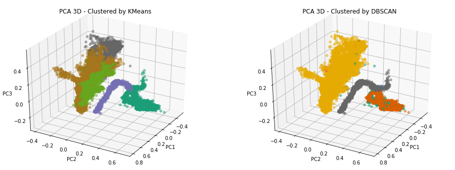
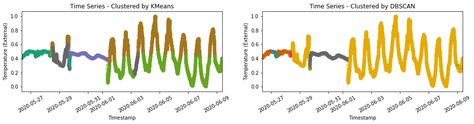
Principal Components Analysis (PCA) is a dimension reduction technique that creates new uncorrelated variables in order to increase interpretability and minimize information loss. In this project, after applying K-means and DBSCAN algorithms on the normalized data, PCA is performed and the clustering results are plotted in both 2D (Figure 7) and 3D (Figure 8) using the first 2 and 3 principal components. In addition, to view the clustering results from another perspective, the labeled time series plots are made, and the Temperature (External) plot is shown in Figure 9 as an example.

主成分分析(PCA)是一種降維技術，可創建新的不相關變量以提高可解釋性并最大程度地減少信息丟失。 在這個項目中，在對標準化數據應用K-means和DBSCAN算法之后，執行PCA，并使用前2個和3個主成分在2D(圖7)和3D(圖8)中繪制聚類結果。 此外，要從另一個角度查看聚類結果，請繪制標記的時間序列圖，并以溫度(外部)圖為例，如圖9所示。

From the plots, it can be clearly seen that both methods are able to distinguish between the indoor/outdoor pattern changes that I mentioned in section 2.1. The main difference is that the partition-based K-means method is more sensitive to the magnitude changes caused by day/night alternation. Many variables in the dataset are subject to such obvious sinusoidal changes that happen at the same time, including Temperature (External and Internal), Humidity (External and internal) and Ozone. K-means tend to treat peaks and valleys differently. On the other hand, density-based DBSCAN cares less about the magnitude difference but pays more attention to the density distributions. Therefore, it clusters the whole sinusoidal part as one mass cloud as seen in Figure 7 and Figure 8.

從圖中可以清楚地看到，兩種方法都能夠區分我在2.1節中提到的室內/室外模式變化。 主要區別在于基于分區的K均值方法對晝夜交替引起的幅度變化更敏感。 數據集中的許多變量會同時發生明顯的正弦變化，包括溫度(外部和內部)，濕度(外部和內部)和臭氧。 K均值傾向于以不同的方式對待峰谷。 另一方面，基于密度的DBSCAN不太關心幅度差異，而更多地關注密度分布。 因此，它將整個正弦曲線部分聚集為一個質量云，如圖7和圖8所示。

It is not possible to comment on which clustering method is better than the other at this stage because they are distinctive enough to function for different interests. If we are more interested in treating the high-low portions of the sinusoidal signals differently, we are going to use K-means; if we only want to distinguish between indoor/outdoor mode, then DBSCAN is better. In addition, since it is an unsupervised learning task, there is no way of quantifying the performance between models except for visualizing and judging by experience. In the future, if some labeled data is provided, the results can be turned into a semi-supervised learning task, and more intuitions can be gained toward model selection.

在此階段，無法評論哪種聚類方法比另一種更好，因為它們具有足夠的獨特性，可以針對不同的利益發揮作用。 如果我們對以不同的方式處理正弦信號的高-低部分更感興趣，我們將使用K-means。 如果我們只想區分室內/室外模式，則DBSCAN更好。 此外，由于這是一項無監督的學習任務，因此除了根據經驗進行可視化和判斷外，無法量化模型之間的性能。 將來，如果提供一些標記的數據，則可以將結果轉換為半監督學習任務，并且可以獲得更多的直覺來進行模型選擇。

4。結論 (4. Conclusion)

In this post, I briefly walk through the approaches and findings of exploratory data analysis and correlation analysis, as well as the constructions of three distinct modeling pipelines that used for point anomaly detection, collective anomaly detection, and clustering.

在本文中，我簡要介紹了探索性數據分析和相關性分析的方法和發現，以及用于點異常檢測，集體異常檢測和聚類的三個不同的建模管道的構建。

In the exploratory data analysis section, the sensor reading time intervals are found to vary severely. Even if most of them are contained around a minute, the inconsistency problem is still worth looking into due to the fact that it might lower the efficiency and performance of analytical tasks. The measuring environment is found subject to changes from the time series plots and later reassured by aligning with the actual Toronto weather data as well as the clustering results. In addition, the correlation between features is studied and exemplified. A few confusions are raised such as the strange relationship between Temperature (Internal) and Temperature (External), which needs to be studied through experiments or the device itself.

在探索性數據分析部分中，發現傳感器讀取時間間隔變化很大。 即使其中大多數都在大約一分鐘之內，但由于不一致的問題可能會降低分析任務的效率和性能，因此仍然值得研究。 發現測量環境可能會隨著時間序列圖的變化而變化，隨后通過與實際的多倫多天氣數據以及聚類結果保持一致來放心。 另外，研究并舉例說明了特征之間的相關性。 引起了一些混亂，例如溫度(內部)和溫度(外部)之間的奇怪關系，需要通過實驗或設備本身進行研究。

In the anomaly detection section, since “system fault” and “external event” are not clearly defined, I split the project into three different tasks. Point anomalies are defined as severely deviated and discontinued data points. The rolling median method is used here to successfully automate the process of labeling such point anomalies. Collective anomalies, on the other hand, are defined as the deviated collection of data points, usually seen as abrupt increases or decreases. This task is accomplished by extracting features from time series data and then training of regression models. Clustering is also performed on the dataset using K-mean and DBSCAN, both of which play to their strength and successfully clustered data by leveraging their similar and dissimilar characteristics.

在異常檢測部分，由于未明確定義“系統故障”和“外部事件”，因此我將項目分為三個不同的任務。 點異常定義為嚴重偏離和中斷的數據點。 這里使用滾動中值法來成功地自動標記此類點異常的過程。 另一方面，集體異常定義為偏離的數據點集合，通常被視為突然增加或減少。 通過從時間序列數據中提取特征，然后訓練回歸模型來完成此任務。 還使用K均值和DBSCAN對數據集執行聚類，兩者均發揮了自己的優勢，并通過利用它們的相似和不同特性成功地對數據進行了聚類。

All of the anomaly detection models introduced in this project are only prototypes without extensive model sections and fine-tunings. There are great potentials for each of them to evolve into better forms if putting more effort and through gaining more knowledge of the data. For point anomalies, there are many more machine-learning-based outlier detection techniques such as isolation forest and local outlier factors to accommodate for more complex data forms. For collective anomaly, state-of-the-art LSTM is worth putting effort into, especially in time series data and sequence modeling. For clustering, there are many other families of methods, such as hierarchical and grid-based clustering. They are capable of achieving similar great performance.

本項目中介紹的所有異常檢測模型只是原型，沒有廣泛的模型部分和微調。 如果付出更多的努力并獲得更多的數據知識，他們每個人都有很大的潛力發展成更好的形式。 對于點異常，還有更多基于機器學習的離群值檢測技術，例如隔離林和局部離群值因素，可以適應更復雜的數據形式。 對于集體異常，值得投入最新的LSTM，特別是在時間序列數據和序列建模方面。 對于群集，還有許多其他方法系列，例如分層和基于網格的群集。 它們能夠實現類似的出色性能。

Of course, these future directions are advised based on the premise of no labeled data. If experienced engineers or scientists are able to give their insights on which types of data are considered as “system fault” or “external event”, more exciting progress will surely be made by transforming the tasks into semi-supervised or supervised learning problems, where more tools will be available to choose.

當然，這些未來的方向是在沒有標簽數據的前提下提出的。 如果經驗豐富的工程師或科學家能夠就哪些數據類型被視為“系統故障”或“外部事件”給出自己的見解，那么將任務轉變為半監督或監督學習問題肯定會取得更加令人興奮的進展。有更多工具可供選擇。