This is series of how to developed data science project.

這是如何開發數據科學項目的系列。

This is part 1.

這是第1部分。

All the Life-cycle In A Data Science Projects-1. Data Analysis and visualization.2. Feature Engineering.3. Feature Selection.4. Model Building.5. Model Deployment.

數據科學項目中的所有生命周期-1 .數據分析和可視化2。 特征工程3。 功能選擇4。 建立模型5。 模型部署。

This whole Data science project life cycle divided into 4 parts.

整個數據科學項目生命周期分為4個部分。

Part 1: How to analysis and visualize the data.

第1部分：如何分析和可視化數據。

Part 2: How to perform feature engineering on data.

第2部分：如何對數據執行特征工程。

Part 3: How to perform feature extraction.

第3部分：如何執行特征提取。

Part 4: model building and development.

第4部分：模型構建和開發。

This tutorial is helpful for them. who has always confused , how to developed data science projects and what is the process for developing data science projects.

本教程對他們有幫助。 誰總是困惑，如何開發數據科學項目以及開發數據科學項目的過程是什么。

So, if you are one of them . so you are at right place.

因此，如果您是其中之一。 所以你來對地方了。

Now, In this whole series. we gonna discuss about complete life cycle of data science projects. we will discuss from Scratch.

現在，在整個系列中。 我們將討論數據科學項目的完整生命周期。 我們將從頭開始進行討論。

In this Part 1. we will see, how to analysis and visualize the data.

在第1部分中，我們將看到如何分析和可視化數據。

So, for all of this, we have to take simple data set of Titanic: Machine Learning from Disaster

因此，對于所有這些，我們必須采用“ 泰坦尼克號：災難中的機器學習”的簡單數據集

So, using this dataset we will see, how complete data science life cycle is work.

因此，使用該數據集，我們將看到完整的數據科學生命周期是如何工作的。

In next future tutorial we will take complex dataset.

在下一個未來的教程中，我們將采用復雜的數據集。

dataset link -https://www.kaggle.com/c/titanic/data

數據集鏈接 -https://www.kaggle.com/c/titanic/data

In this dataset 891 records with 11 features(columns).

在該數據集中，有11個特征(列)的891條記錄。

So, let begin with part 1-Analysis and visualize the data in data science life cycle.

因此，讓我們從第1部分開始分析，并可視化數據科學生命周期中的數據。

STEP 1-

第1步-

import pandas as pd
import numpy as np
import matplotlib as plt
%matplotlib inline

Import pandas for perform manipulation on dataset.

導入熊貓以對數據集執行操作 。

Import numpy to deal with mathematical operations.

導入numpy以處理數學運算 。

Import matplotlib for visualize the dataset in form of graphs.

導入matplotlib在圖表的形式直觀的數據集。

STEP 2-

第2步-

data=pd.read_csv(‘path.csv’)
data.head(5)

Dataset is like this-

數據集是這樣的-

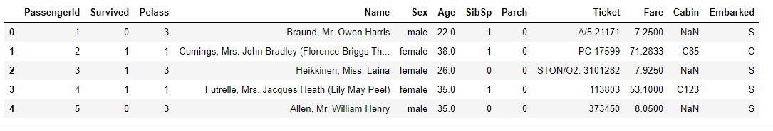
There is 11 features in dataset.

數據集中有11個要素。

1-PassengerId

1-PassengerId

2-Pclass

2類

3-Name

3名

4-Sex

4性別

5-Age

5歲

6-Sibsp

6麻痹

7-Parch

7月

8-Ticket

8票

9-Fare

9票價

10-cabin

10艙

11-embeded

11嵌入式

ABOUT THE DATA –

關于數據–

VariableDefinitionKeysurvivalSurvival0 = No, 1 = YespclassTicket class1 = 1st, 2 = 2nd, 3 = 3rdsexSexAgeAge in yearssibsp# of siblings / spouses aboard the Titanicparch# of parents / children aboard the TitanicticketTicket numberfarePassenger farecabinCabin numberembarkedPort of EmbarkationC = Cherbourg, Q = Queenstown, S = Southampton

VariableDefinitionKeysurvivalSurvival0 =否，1 = YespclassTicket class1 = 1st，2 = 2nd，3 = 3rdsexSexAgeAge年齡在Titanicparch的同胞/配偶中的同胞/配偶數＃TitanicticketTicket的票價/乘客乘母票的票價是南安普敦

可變音符 (Variable Notes)

pclass: A proxy for socio-economic status (SES)1st = Upper2nd = Middle3rd = Lower

pclass ：社會經濟地位(SES)的代理人1st =上層2nd =中間3rd =下層

age: Age is fractional if less than 1. If the age is estimated, is it in the form of xx.5

age ：年齡小于1時是小數。如果估計了年齡，則以xx.5的形式出現

sibsp: The dataset defines family relations in this way…Sibling = brother, sister, stepbrother, stepsisterSpouse = husband, wife (mistresses and fiancés were ignored)

sibsp ：數據集通過這種方式定義家庭關系… 兄弟姐妹 =兄弟，姐妹，繼兄弟，繼母配偶 =丈夫，妻子(情婦和未婚夫被忽略)

parch: The dataset defines family relations in this way…Parent = mother, fatherChild = daughter, son, stepdaughter, stepsonSome children travelled only with a nanny, therefore parch=0 for them.

parch ：數據集通過這種方式定義家庭關系… 父母 =母親，父親孩子 =女兒，兒子，繼女，繼子有些孩子只帶保姆旅行，因此parch = 0。

STEP 3 -After import the dataset. now time to analysis the data.

步驟3-導入數據集后。 現在該分析數據了。

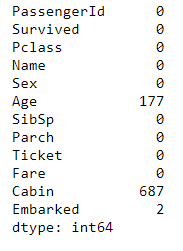
First, we gonna go check the Null value in dataset.

首先，我們要檢查數據集中的Null值。

null_count=data.isnull().sum()null_count

In that code-

在該代碼中-

Now here, We are checking, how many features contains null values.

現在在這里，我們正在檢查多少個功能包含空值。

here is list..

這是清單。

STEP 4-

第4步-

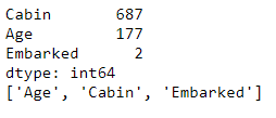
null_features=null_count[null_count>0].sort_values(ascending=False)
print(null_features) 
null_features=[features for features in data.columns if data[features].isnull().sum()>0]
print(null_features)

In 1st line of code – we are extracting only those features with their null values , who has contains 1 or more than 1 Null values.

在第一行代碼中，我們僅提取具有零值的特征 ，這些特征包含1個或多個1個 Null值。

In 2nd line of code – print those features, who has contains 1 or more than 1 null values.

在第二行代碼中–打印那些包含1個或多個1個空值的要素。

In 3rd line of code – we extracting only those features, who has contains 1 or more than 1 null values using list comprehensions.

在代碼的第三行中，我們僅使用列表推導提取那些包含1個或多個1個空值的要素 。

In 4th line of code -Print those all features.

在代碼的第4行-P rint所有這些功能。

We will deal with null values in feature engineering part 2.

我們將在要素工程第2部分中處理空值。

STEP 5-

步驟5

data.shape

Check the shape of the dataset.

檢查數據集的形狀。

STEP 6 - Check unique values in passenger i’d, name, ticket columns.

第6步-檢查乘客編號， 姓名 ， 機票欄中的唯一值。

print("{} unique values in passenger id columns ".format(len(data.PassengerId.unique())))
print("{} unique values in Name columns ".format(len(data.Name.unique())))
print("{} unique values in Ticket columns ".format(len(data.Ticket.unique())))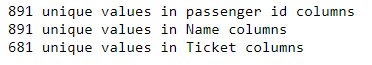

891 unique values in passenger id and name columns

乘客ID和名稱列中的891個唯一值

681 unique values in ticket columns.

憑單列中有681個唯一值。

So , These three columns will not be do any effect on our prediction. these columns not useful, because all values are unique values .so we are dropping these three columns from the dataset.

因此，這三列將不會對我們的預測產生任何影響。 這些列沒有用，因為所有值都是唯一值。因此我們從數據集中刪除了這三列 。

STEP 7- Drop these three columns

步驟7-刪除這三列

data=data.drop(['PassengerId','Name','Ticket'],axis=1)

STEP 8-

步驟8

data.shape

Check the shape of dataframe once again .It has 891 *9.

再次檢查數據框的形狀。它具有891 * 9。

Now, After drop three features .9 columns (features) present in dataset.

現在，刪除三個功能。 數據集中存在9列 ( 特征 )。

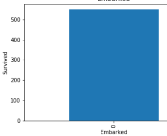
STEP 9 - In this step, we gonna go check is this dataset is balance or not.

步驟9-在這一步中 ，我們將檢查此數據集是否平衡。

If dataset is not balance . it might be reason of bad accuracy, because in dataset. if you have many data points which belong only to single class. so this thing may lead over-fitting problem.

如果數據集不平衡。 這可能是因為數據集中的準確性不佳 。 如果您有許多僅屬于單個類的數據點。 所以這東西可能會導致過度擬合的問題。

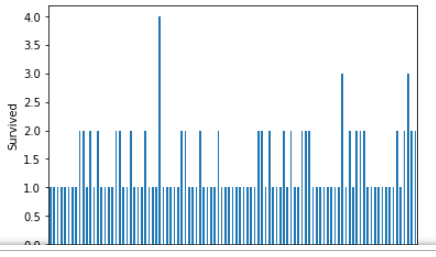
data["Survived"].value_counts().plot(kind='bar')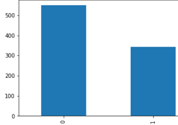

Here, Dataset is not proper balance, it’s 60–40 ratio.

這里 ，數據集不是適當的平衡， 它是60–40的比率。

So , it will not be effect so much on our predictions. If it effect on our prediction we will deal with this soon.

因此，它對我們的預測影響不大。 如果它影響我們的預測， 我們將盡快處理。

STEP 10 -

步驟10-

datasett=data.copy
not_survived=data[data['Survived']==0]survived=data[data['Survived']==1]

1st line of code — Copy the dataset in dataset variable. because , we will perform some manipulation on data . so that manipulation does not effect on real data. so that we are copying dataset into datasett variable.

第一行代碼—將數據集復制到數據集變量中。 因為，我們將對數據進行一些處理 。 這樣操作就不會影響真實數據。 所以，我們要復制的數據集到datasett變量。

2nd line of code - we are dividing dependent feature (“Survived “) into two part-

代碼的第二行-我們將依存特征(“幸存的”)分為兩部分，

1. extract all non survival data points from the “Survived” column and store into not_survived variable.

1.從“生存”列中提取所有非生存數據點，并將其存儲到not_survived變量中。

2. extract all survival data points from the “Survived” column and store into survival variable.

2.從“ Survived”列中提取所有生存數據點，并將其存儲到生存變量中。

It is for visualize the dataset.

用于可視化數據集。

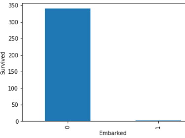
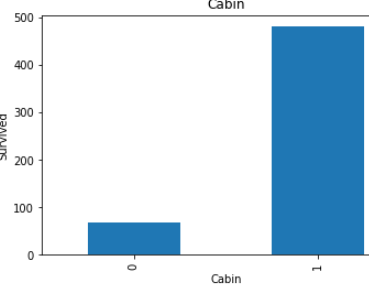
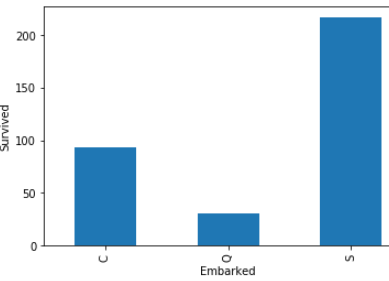
STEP 11 - Now , We are checking of null values’s features(columns) dependency with the Survived or non survived peoples .

步驟11-現在 ，我們正在與生存或未生存的人一起檢查空值的特征 ( 列 ) 依賴性 。

First of all , right here, we are checking null values ‘s features(columns) dependency with survived people only.

首先，在這里，我們僅與幸存者一起檢查null值的功能(列)依賴性。

import matplotlib.pyplot as plt
dataset = survived.copy()%matplotlib inline 
for features in null_features:
    dataset[features] = np.where(dataset[features].isnull(), 1, 0)
    dataset.groupby(features)['Survived'].count().plot.bar()
    plt.xlabel(features)
    plt.ylabel('Survived')
    plt.title(features)
    plt.show()

1st line of code- Import matplotlib.lib for visualize purpose.

第一行代碼-我導入matplotlib.lib以實現可視化目的。

2nd line of code- copy the only survived people dataset into dataset variable for further processing and it copy because any manipulation does not effect on real data frame.

代碼的第二行-將唯一幸存的人員數據集復制到數據集變量中以進行進一步處理， 并進行復制，因為任何操作都不會影響實際數據幀。

3rd line of code - Used loop . This loop will take only null value’s features(columns) only.

第三行代碼-使用循環 。 此循環將僅采用空值的功能(列)。

4th line of code — Null values replace by the 1 or non null values replace by 0. for check the dependency.

代碼的第四行- 空值替換為1或非空值替換為0 。 用于檢查依賴性 。

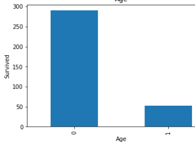
Look in above graphs . all 1 values is basically null values and 0 values is not null values.

看上面的圖表 。 所有1個值基本上都是空值，而0個值不是空值。

In age’s graph , dependency is low with null value .

在age的圖中，依賴性較低，值為null。

In cabin’s graph, dependency is high with null values.

在機艙的圖形中，具有空值的依賴性較高。

In embarked’s graph ,there is approximate not any dependency with null values.

在圖的圖形中，沒有近似值的依賴項為空。

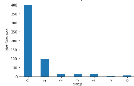
STEP 12- Over here, we are checking dependency with not survived peoples.

第12步-在這里， 我們正在檢查對尚未幸存的民族的依賴性。

import matplotlib.pyplot as plt
dataset = not_survived.copy()
%matplotlib inline 
for features in null_features:
    dataset = not_survived.copy()
    dataset[features] = np.where(dataset[features].isnull(), 1, 0)
    dataset.groupby(features)['Survived'].count().plot.bar()
    plt.xlabel(features)
    plt.ylabel('Survived')
    plt.title(features)
    plt.show()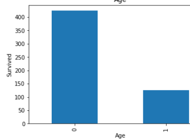

Same like step 7 . but over here we are dealing with non survival people’s.

與步驟7相同。 但在這里，我們正在與非生存者打交道。

STEP 13 -Let find the relationship between all categories variable(features) with survive peoples.

步驟13-讓我們找出所有類別變量 (特征)與生存人群之間的關系。

num_features=data.columns
for feature in num_features:
    if feature != 'Survived' and feature !='Fare' and feature != 'Age':
        survived.groupby(feature)['Survived'].count().plot.bar()
        plt.xlabel(feature)
        plt.ylabel('Survived')
        plt.title(feature)
        plt.show()

Survived is dependent variable (feature).

生存的是因變量(特征)。

Fare is numeric variable.

票價是數字變量。

Age is also numeric variable.

年齡也是數字變量。

So , we are not considering these three features (columns) .

因此 ，我們不考慮這三個功能 ( 列 )。

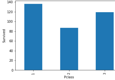
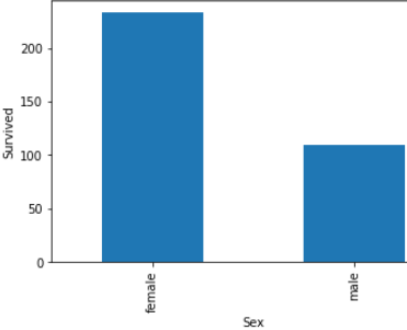
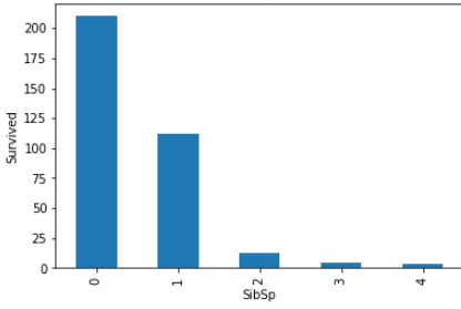
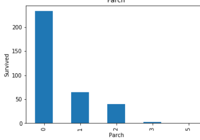
These all are relationship between categorical variables(features) with survived peoples.

這些都是類別變量 ( 特征 )與幸存者之間的關系 。

STEP 14- Let find the relationship between all categories variable with not survived peoples.

步驟14-讓所有類別的變量與沒有生存的人之間建立關系 。

for feature in num_features:
    if feature != 'Survived' and feature !='Fare' and feature != 'Age':
        not_survived.groupby(feature)['Survived'].count().plot.bar()
        plt.xlabel(feature)
        plt.ylabel('Not Survived')
        plt.title(feature)
        plt.show()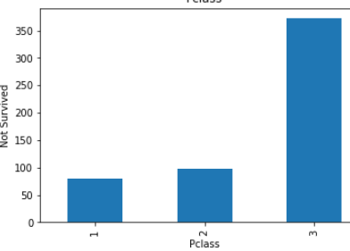

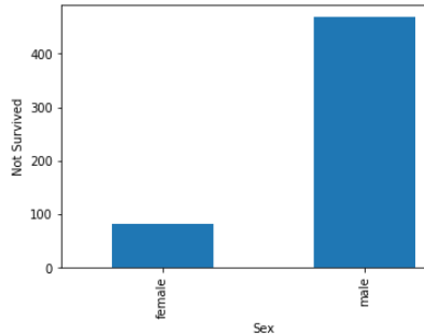
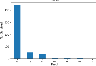
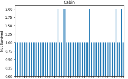
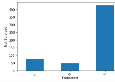
These all are relationship between categorical variables(features) with not survived peoples.

這些都是沒有生存的人的 分類變量 ( 特征 )之間的關系 。

STEP 15 -Now check with the numeric variables.

步驟15-現在檢查數字變量 。

non_sur_fare_mean=round(not_survived['Fare'].mean())
non_sur_age_mean=round(not_survived['Age'].mean())  
print('its not survived people fare averages',non_sur_fare_mean)
print('its not survived people Age averages',non_sur_age_mean)sur_fare_mean=round(survived['Fare'].mean())
sur_age_mean=round(survived['Age'].mean())  
print('its survived people fare averages',sur_fare_mean)
print('its survived people Age averages',sur_age_mean)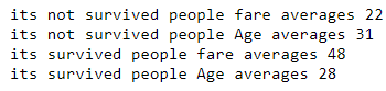

From this , Its clearly show-

由此可見，它清楚地表明：

Those who were above 31 years old had very few chances to escapes.

那些31歲以上的人很少有機會逃脫。

Those who fares was less than 48 had very few chances to escapes.

票價低于48美元的人幾乎沒有機會逃脫。

STEP 16- Analysis the numeric features. check distribution of the numeric variable(features).

步驟16- 分析 數字特征 。 檢查數字變量的 分布 ( 功能 )。

for feature in num_features:
    if feature =='Fare' or feature == 'Age':
        data[feature].hist(bins=25)
        plt.xlabel(feature)
        plt.ylabel("Count")
        plt.title(feature)
        plt.show()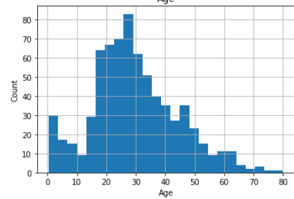

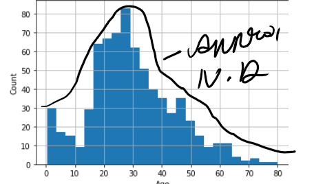
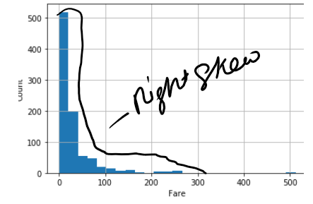
Age followed normal distribution, but Fare is not following normal distribution.

年齡遵循正態分布 ，但票價不遵循正態分布 。

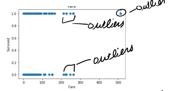
STEP 17- Check the outliers in dataset.

步驟17-檢查數據集中的離群值 。

There are many ways to check the outliers.

有許多方法可以檢查異常值。

1- Box plot.

1-盒圖。

2- Z-score.

2-Z得分。

3- scatter plot

3-散點圖

ETC.

等等。

First of all , Find the outliers using scatter plot-

首先，使用散點圖找到離群值-

for feature in num_features:
        if feature =='Fare' or feature == 'Age':plt.scatter(data[feature],data['Survived'])
                plt.xlabel(feature)
                plt.ylabel('Survived')
                plt.title(feature)
                plt.show()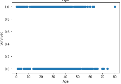

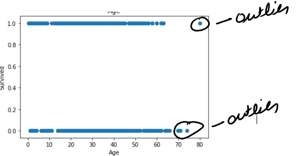
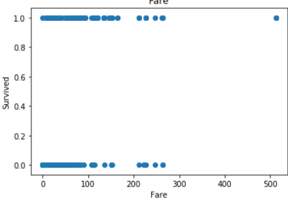
In Age less no of outlier.

在年齡中，沒有異常值。

but in fare you can see there is lot of outlier in fare.

但是在票價上您可以看到票價中有很多離群值。

STEP 18- Find outlier using box plot-

步驟18- 使用箱形圖查找離群值-

Box plot is better way to check outlier in distribution.

箱形圖是檢查分布中異常值的更好方法。

for feature in num_features:
    if feature =='Fare' or feature == 'Age':
            data.boxplot(column=feature)
            plt.ylabel(feature)
            plt.title(feature)
            plt.show()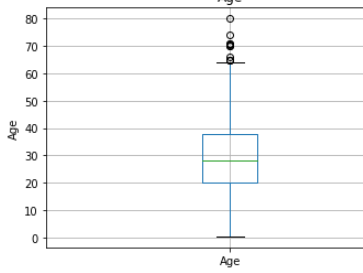

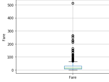
Box plot is also show same picture like scatter.

箱形圖也顯示散點圖。

Age has few no of outlier , but in fare has lot of outliers.

年齡很少有異常值，但票價中有很多異常值。

This first part ended here.

第一部分到此結束。

In this part we saw. how, we can analysis and visualize the dataset.

在這一部分中，我們看到了。 如何分析和可視化數據集。

In next part we will see how feature engineering perform.

在下一部分中，我們將了解要素工程的性能。