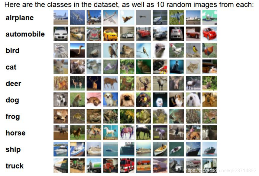
Cifar-10數據集包含10類共60000張32*32的彩色圖片，每類6000張圖。包括50000張訓練圖片和 10000張測試圖片

代碼分為數據處理部分和卷積網絡訓練部分：

數據處理部分：

#該文件負責讀取Cifar-10數據并對其進行數據增強預處理
import os
import tensorflow as tf
num_classes=10#設定用于訓練和評估的樣本總數
num_examples_pre_epoch_for_train=50000
num_examples_pre_epoch_for_eval=10000#定義一個空類，用于返回讀取的Cifar-10的數據
class CIFAR10Record(object):pass#定義一個讀取Cifar-10的函數read_cifar10()，這個函數的目的就是讀取目標文件里面的內容
def read_cifar10(file_queue):result=CIFAR10Record()label_bytes=1                                            #標簽占用一字節，如果是Cifar-100數據集，則此處為2result.height=32result.width=32result.depth=3                                           #因為是RGB三通道，所以深度是3image_bytes=result.height * result.width * result.depth  #圖片樣本總元素數量record_bytes=label_bytes + image_bytes                   #因為每一個樣本包含圖片和標簽，所以最終的元素數量還需要圖片樣本數量加上一個標簽值reader=tf.FixedLengthRecordReader(record_bytes=record_bytes)  #使用tf.FixedLengthRecordReader()創建一個文件讀取類。該類的目的就是讀取文件result.key,value=reader.read(file_queue)                 #使用該類的read()函數從文件隊列里面讀取文件record_bytes=tf.decode_raw(value,tf.uint8)               #讀取到文件以后，將讀取到的文件內容從字符串形式解析為圖像對應的像素數組#因為該數組第一個元素是標簽，所以我們使用strided_slice()函數將標簽提取出來，并且使用tf.cast()函數將這一個標簽轉換成int32的數值形式result.label=tf.cast(tf.strided_slice(record_bytes,[0],[label_bytes]),tf.int32)#剩下的元素再分割出來，這些就是圖片數據，因為這些數據在數據集里面存儲的形式是depth * height * width，我們要把這種格式轉換成[depth,height,width]#這一步是將一維數據轉換成3維數據depth_major=tf.reshape(tf.strided_slice(record_bytes,[label_bytes],[label_bytes + image_bytes]),[result.depth,result.height,result.width])  #我們要將之前分割好的圖片數據使用tf.transpose()函數轉換成為高度信息、寬度信息、深度信息這樣的順序#這一步是轉換數據排布方式，變為(h,w,c)result.uint8image=tf.transpose(depth_major,[1,2,0])return result                                 #返回值是已經把目標文件里面的信息都讀取出來def inputs(data_dir,batch_size,distorted):               #這個函數就對數據進行預處理---對圖像數據是否進行增強進行判斷，并作出相應的操作filenames=[os.path.join(data_dir,"data_batch_%d.bin"%i)for i in range(1,6)]   #拼接地址file_queue=tf.train.string_input_producer(filenames)     #根據已經有的文件地址創建一個文件隊列read_input=read_cifar10(file_queue)                      #根據已經有的文件隊列使用已經定義好的文件讀取函數read_cifar10()讀取隊列中的文件reshaped_image=tf.cast(read_input.uint8image,tf.float32)   #將已經轉換好的圖片數據再次轉換為float32的形式num_examples_per_epoch=num_examples_pre_epoch_for_trainif distorted != None:                         #如果預處理函數中的distorted參數不為空值，就代表要進行圖片增強處理cropped_image=tf.random_crop(reshaped_image,[24,24,3])          #首先將預處理好的圖片進行剪切，使用tf.random_crop()函數flipped_image=tf.image.random_flip_left_right(cropped_image)    #將剪切好的圖片進行左右翻轉，使用tf.image.random_flip_left_right()函數adjusted_brightness=tf.image.random_brightness(flipped_image,max_delta=0.8)   #將左右翻轉好的圖片進行隨機亮度調整，使用tf.image.random_brightness()函數adjusted_contrast=tf.image.random_contrast(adjusted_brightness,lower=0.2,upper=1.8)    #將亮度調整好的圖片進行隨機對比度調整，使用tf.image.random_contrast()函數float_image=tf.image.per_image_standardization(adjusted_contrast)          #進行標準化圖片操作，tf.image.per_image_standardization()函數是對每一個像素減去平均值并除以像素方差float_image.set_shape([24,24,3])                      #設置圖片數據及標簽的形狀read_input.label.set_shape([1])min_queue_examples=int(num_examples_pre_epoch_for_eval * 0.4)print("Filling queue with %d CIFAR images before starting to train.    This will take a few minutes."%min_queue_examples)images_train,labels_train=tf.train.shuffle_batch([float_image,read_input.label],batch_size=batch_size,num_threads=16,capacity=min_queue_examples + 3 * batch_size,min_after_dequeue=min_queue_examples,)#使用tf.train.shuffle_batch()函數隨機產生一個batch的image和labelreturn images_train,tf.reshape(labels_train,[batch_size])else:                               #不對圖像數據進行數據增強處理resized_image=tf.image.resize_image_with_crop_or_pad(reshaped_image,24,24)   #在這種情況下，使用函數tf.image.resize_image_with_crop_or_pad()對圖片數據進行剪切float_image=tf.image.per_image_standardization(resized_image)          #剪切完成以后，直接進行圖片標準化操作float_image.set_shape([24,24,3])read_input.label.set_shape([1])min_queue_examples=int(num_examples_per_epoch * 0.4)images_test,labels_test=tf.train.batch([float_image,read_input.label],batch_size=batch_size,num_threads=16,capacity=min_queue_examples + 3 * batch_size)#這里使用batch()函數代替tf.train.shuffle_batch()函數return images_test,tf.reshape(labels_test,[batch_size])

卷積網絡訓練部分：

#該文件的目的是構造神經網絡的整體結構，并進行訓練和測試（評估）過程
import tensorflow as tf
import numpy as np
import time
import math
import Cifar10_datamax_steps=4000
batch_size=100
num_examples_for_eval=10000
data_dir="Cifar_data/cifar-10-batches-bin"#創建一個variable_with_weight_loss()函數，該函數的作用是：
#   1.使用參數w1控制L2 loss的大小
#   2.使用函數tf.nn.l2_loss()計算權重L2 loss
#   3.使用函數tf.multiply()計算權重L2 loss與w1的乘積，并賦值給weights_loss
#   4.使用函數tf.add_to_collection()將最終的結果放在名為losses的集合里面，方便后面計算神經網絡的總體loss，
def variable_with_weight_loss(shape,stddev,w1):var=tf.Variable(tf.truncated_normal(shape,stddev=stddev))if w1 is not None:weights_loss=tf.multiply(tf.nn.l2_loss(var),w1,name="weights_loss")tf.add_to_collection("losses",weights_loss)return var#使用上一個文件里面已經定義好的文件序列讀取函數讀取訓練數據文件和測試數據從文件.
#其中訓練數據文件進行數據增強處理，測試數據文件不進行數據增強處理
images_train,labels_train=Cifar10_data.inputs(data_dir=data_dir,batch_size=batch_size,distorted=True)
images_test,labels_test=Cifar10_data.inputs(data_dir=data_dir,batch_size=batch_size,distorted=None)#創建x和y_兩個placeholder，用于在訓練或評估時提供輸入的數據和對應的標簽值。
#要注意的是，由于以后定義全連接網絡的時候用到了batch_size，所以x中，第一個參數不應該是None，而應該是batch_size
x=tf.placeholder(tf.float32,[batch_size,24,24,3])
y_=tf.placeholder(tf.int32,[batch_size])#創建第一個卷積層 shape=(kh,kw,ci,co)
kernel1=variable_with_weight_loss(shape=[5,5,3,64],stddev=5e-2,w1=0.0)
conv1=tf.nn.conv2d(x,kernel1,[1,1,1,1],padding="SAME")
bias1=tf.Variable(tf.constant(0.0,shape=[64]))
relu1=tf.nn.relu(tf.nn.bias_add(conv1,bias1))
pool1=tf.nn.max_pool(relu1,ksize=[1,3,3,1],strides=[1,2,2,1],padding="SAME")#創建第二個卷積層
kernel2=variable_with_weight_loss(shape=[5,5,64,64],stddev=5e-2,w1=0.0)
conv2=tf.nn.conv2d(pool1,kernel2,[1,1,1,1],padding="SAME")
bias2=tf.Variable(tf.constant(0.1,shape=[64]))
relu2=tf.nn.relu(tf.nn.bias_add(conv2,bias2))
pool2=tf.nn.max_pool(relu2,ksize=[1,3,3,1],strides=[1,2,2,1],padding="SAME")#因為要進行全連接層的操作，所以這里使用tf.reshape()函數將pool2輸出變成一維向量，并使用get_shape()函數獲取扁平化之后的長度
reshape=tf.reshape(pool2,[batch_size,-1])    #這里面的-1代表將pool2的三維結構拉直為一維結構
dim=reshape.get_shape()[1].value             #get_shape()[1].value表示獲取reshape之后的第二個維度的值#建立第一個全連接層
weight1=variable_with_weight_loss(shape=[dim,384],stddev=0.04,w1=0.004)
fc_bias1=tf.Variable(tf.constant(0.1,shape=[384]))
fc_1=tf.nn.relu(tf.matmul(reshape,weight1)+fc_bias1)#建立第二個全連接層
weight2=variable_with_weight_loss(shape=[384,192],stddev=0.04,w1=0.004)
fc_bias2=tf.Variable(tf.constant(0.1,shape=[192]))
local4=tf.nn.relu(tf.matmul(fc_1,weight2)+fc_bias2)#建立第三個全連接層
weight3=variable_with_weight_loss(shape=[192,10],stddev=1 / 192.0,w1=0.0)
fc_bias3=tf.Variable(tf.constant(0.1,shape=[10]))
result=tf.add(tf.matmul(local4,weight3),fc_bias3)#計算損失，包括權重參數的正則化損失和交叉熵損失
cross_entropy=tf.nn.sparse_softmax_cross_entropy_with_logits(logits=result,labels=tf.cast(y_,tf.int64))weights_with_l2_loss=tf.add_n(tf.get_collection("losses"))
loss=tf.reduce_mean(cross_entropy)+weights_with_l2_losstrain_op=tf.train.AdamOptimizer(1e-3).minimize(loss)#函數tf.nn.in_top_k()用來計算輸出結果中top k的準確率，函數默認的k值是1，即top 1的準確率，也就是輸出分類準確率最高時的數值
top_k_op=tf.nn.in_top_k(result,y_,1)init_op=tf.global_variables_initializer()
with tf.Session() as sess:sess.run(init_op)#啟動線程操作，這是因為之前數據增強的時候使用train.shuffle_batch()函數的時候通過參數num_threads()配置了16個線程用于組織batch的操作tf.train.start_queue_runners()      #每隔100step會計算并展示當前的loss、每秒鐘能訓練的樣本數量、以及訓練一個batch數據所花費的時間for step in range (max_steps):start_time=time.time()image_batch,label_batch=sess.run([images_train,labels_train])_,loss_value=sess.run([train_op,loss],feed_dict={x:image_batch,y_:label_batch})duration=time.time() - start_timeif step % 100 == 0:examples_per_sec=batch_size / durationsec_per_batch=float(duration)print("step %d,loss=%.2f(%.1f examples/sec;%.3f sec/batch)"%(step,loss_value,examples_per_sec,sec_per_batch))#計算最終的正確率num_batch=int(math.ceil(num_examples_for_eval/batch_size))  #math.ceil()函數用于求整true_count=0total_sample_count=num_batch * batch_size#在一個for循環里面統計所有預測正確的樣例個數for j in range(num_batch):image_batch,label_batch=sess.run([images_test,labels_test])predictions=sess.run([top_k_op],feed_dict={x:image_batch,y_:label_batch})true_count += np.sum(predictions)#打印正確率信息print("accuracy = %.3f%%"%((true_count/total_sample_count) * 100))

實現結果：

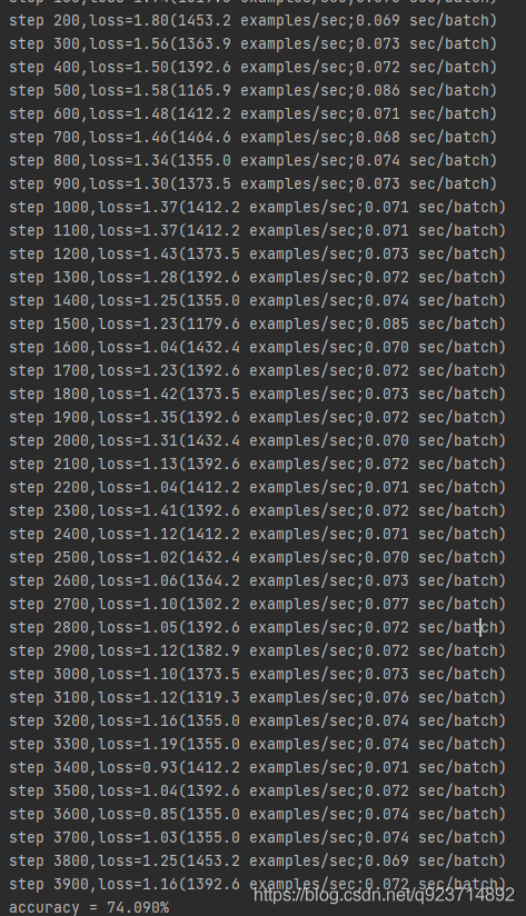
準確率在74%