Pandas is the go-to Python library for data analysis and manipulation. It provides numerous functions and methods that expedice the data analysis process.

Pandas是用于數據分析和處理的Python庫。 它提供了加速數據分析過程的眾多功能和方法。

When it comes to data visualization, pandas is not the prominent choice because there exist great visualization libraries such as matplotlib, seaborn, and plotly.

在數據可視化方面，大熊貓并不是首選，因為存在強大的可視化庫，例如matplotlib，seaborn和plotly。

With that being said, we cannot just ignore the plotting tools of pandas. They help to discover relations within dataframes or series and syntax is pretty simple. Very informative plots can be created with just one line of code.

話雖如此，我們不能僅僅忽略熊貓的繪圖工具。 它們有助于發現數據框或序列中的關系，語法非常簡單。 只需一行代碼就可以創建非常有用的圖。

In this post, we will cover 6 plotting tools of pandas which definitely add value to the exploratory data analysis process.

在本文中，我們將介紹6種熊貓繪圖工具，這些工具肯定會為探索性數據分析過程增添價值。

The first step to create a great machine learning model is to explore and understand the structure and relations within the data.

創建出色的機器學習模型的第一步是探索和理解數據內的結構和關系。

These 6 plotting tools will help you understand the data better:

這6種繪圖工具將幫助您更好地理解數據：

• Scatter matrix plot

  散點圖

• Density plot

  密度圖

• Andrews curves

  安德魯斯曲線

• Parallel coordinates

  平行坐標

• Lag plots

  滯后圖

• Autocorrelation plot

  自相關圖

I will use a diabetes dataset available on kaggle. Let’s first read the dataset into a pandas dataframe.

我將使用kaggle上提供的糖尿病數據集 。 首先讓我們將數據集讀入pandas數據框。

import pandas as pd
import numpy as npimport matplotlib.pyplot as plt
%matplotlib inlinedf = pd.read_csv("/content/diabetes.csv")
print(df.shape)
df.head()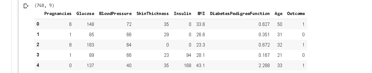

The dataset contains 8 numerical features and a target variable indicating if the person has diabetes.

該數據集包含8個數字特征和一個指示該人是否患有糖尿病的目標變量。

1.散點圖 (1. Scatter matrix plot)

Scatter plots are typically used to explore the correlation between two variables (or features). The values of data points are shown using the cartesian coordinates.

散點圖通常用于探索兩個變量(或特征)之間的相關性。 使用笛卡爾坐標顯示數據點的值。

Scatter plot matrix produces a grid of scatter plots with just one line of code.

散點圖矩陣僅用一行代碼即可生成散點圖的網格。

from pandas.plotting import scatter_matrixsubset = df[['Glucose','BloodPressure','Insulin','Age']]scatter_matrix(subset, figsize=(10,10), diagonal='hist')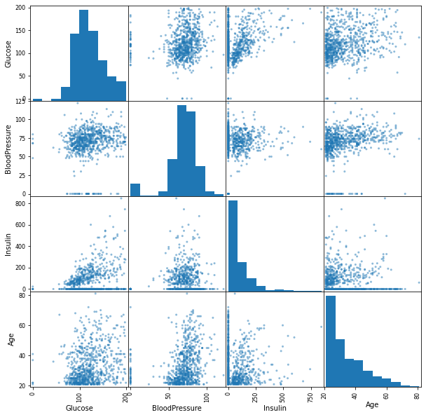

I’ve selected a subset of the dataframe with 4 features for demonstration purposes. The diagonal shows the histogram of each variable but we can change it to show kde plot by setting diagonal parameter as ‘kde’.

為了演示目的，我選擇了具有4個功能的數據框的子集。 對角線顯示每個變量的直方圖，但我們可以通過將對角線參數設置為' kde '來更改它以顯示kde圖。

2.密度圖 (2. Density plot)

We can produce density plots using kde() function on series or dataframe.

我們可以在系列或數據框上使用kde()函數生成密度圖。

subset = df[['Glucose','BloodPressure','BMI']]subset.plot.kde(figsize=(12,6), alpha=1)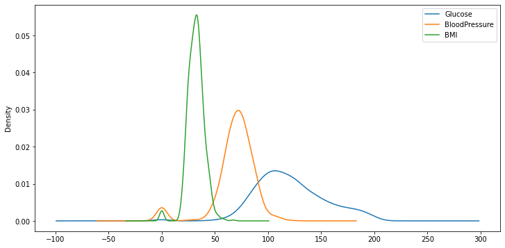

We are able to see the distribution of features with one line of code. Alpha parameter is used to adjust the darkness of lines.

我們可以用一行代碼看到功能的分布。 Alpha參數用于調整線條的暗度。

3.安德魯斯曲線 (3. Andrews curves)

Andrews curves, named after the statistician David F. Andrews, is a tool to plot multivariate data with lots of curves. The curves are created using the attributes (features) of samples as coefficients of Fourier series.

以統計學家大衛·安德魯斯(David F. 使用樣本的屬性(特征)作為傅立葉級數的系數來創建曲線。

We get an overview of clustering of different classes by coloring the curves that belong to each class differently.

我們通過對屬于每個類別的曲線進行不同的著色來獲得對不同類別的聚類的概述。

from pandas.plotting import andrews_curvesplt.figure(figsize=(12,8))subset = df[['Glucose','BloodPressure','BMI', 'Outcome']]andrews_curves(subset, 'Outcome', colormap='Paired')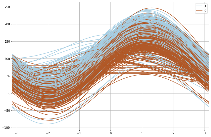

We need to pass a dataframe and name of the variable that hold class information. Colormap parameter is optional. There seems to be a clear distinction (with some exceptions) between 2 classes based on the features in subset.

我們需要傳遞一個保存類信息的數據框和變量名。 Colormap參數是可選的。 根據子集中的功能，兩個類之間似乎有明顯的區別(有些例外)。

4.平行坐標 (4. Parallel coordinates)

Parallel coordinates is another tool for plotting multivariate data. Let’s first create the plot and then talk about what it tells us.

平行坐標是另一個用于繪制多元數據的工具。 讓我們首先創建情節，然后談論它告訴我們的內容。

from pandas.plotting import parallel_coordinatescols = ['Glucose','BloodPressure','BMI', 'Age']plt.figure(figsize=(12,8))parallel_coordinates(df,'Outcome',color=['Blue','Gray'],cols=cols)

We first import parallel_coordinates from pandas plotting tools. Then create a list of columns to use. Then a matplotlib figure is created. The last line creates parallel coordinates plot. We pass a dataframe and name of the class variable. Color parameter is optional and used to determine colors for each class. Finally cols parameter is used to select columns to be used in the plot. If not specified, all columns are used.

我們首先從熊貓繪圖工具導入parallel_coordinates 。 然后創建要使用的列的列表。 然后創建一個matplotlib圖形。 最后一行創建平行坐標圖。 我們傳遞一個數據框和類變量的名稱。 Color參數是可選的，用于確定每個類的顏色。 最后， cols參數用于選擇要在繪圖中使用的列。 如果未指定，則使用所有列。

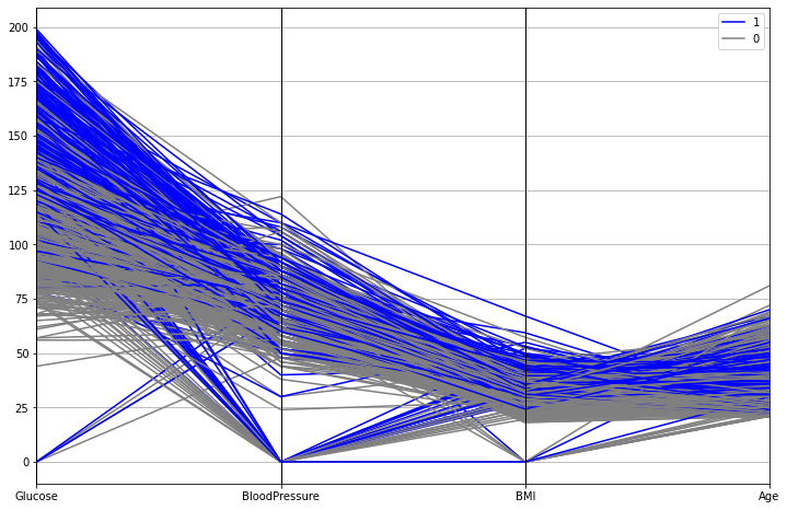
Each column is represented with a vertical line. The horizontal lines represent data points (rows in dataframe). We get an overview of how classes are separated according to features. “Glucose” variable seems to a good predictor to separate these two classes. On the other hand, lines of different classes overlap on “BloodPressure” which indicates it does not perform well in separating the classes.

每列均以垂直線表示。 水平線代表數據點(數據幀中的行)。 我們對如何根據功能分離類進行了概述。 “葡萄糖”變量似乎是區分這兩個類別的良好預測指標。 另一方面，不同類別的行在“ BloodPressure”上重疊，這表明在分隔類別時效果不佳。

5.滯后圖 (5. Lag plot)

Lag plots are used to check the randomness in a data set or time series. If a structure is displayed in lag plot, we can conclude that the data is not random.

滯后圖用于檢查數據集或時間序列中的隨機性。 如果在滯后圖中顯示結構，則可以得出結論，數據不是隨機的。

from pandas.plotting import lag_plotplt.figure(figsize=(10,6))lag_plot(df)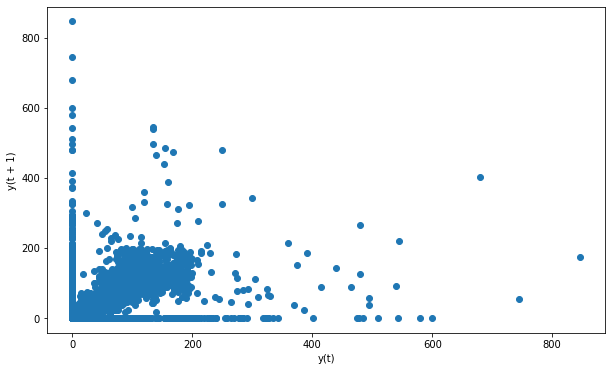

There is no structure in our data set that indicates randomness.

我們的數據集中沒有任何結構表明隨機性。

Let’s see an example of non-random data. I will use the synthetic sample in pandas documentation page.

讓我們看一個非隨機數據的例子。 我將在pandas文檔頁面中使用合成樣本。

spacing = np.linspace(-99 * np.pi, 99 * np.pi, num=1000)data = pd.Series(0.1 * np.random.rand(1000) + 0.9 * np.sin(spacing))plt.figure(figsize=(10,6))lag_plot(data)

We can clearly see a structure on lag plot so the data is not random.

我們可以清楚地看到滯后圖上的結構，因此數據不是隨機的。

6.自相關圖 (6. Autocorrelation plot)

Autocorrelation plots are used to check the randomness in time series. They are produced by calculating the autocorrelations for data values at varying time lags.

自相關圖用于檢查時間序列中的隨機性。 它們是通過計算在不同時滯下數據值的自相關來產生的。

Lag is the time difference. If the autocorrelations are very close to zero for all time lags, the time series is random.

滯后是時差。 如果對于所有時滯，自相關都非常接近零，則時間序列是隨機的。

If we observe one or more significantly non-zero autocorrelations, then we can conclude that time series is not random.

如果我們觀察到一個或多個顯著的非零自相關，則可以得出時間序列不是隨機的結論。

Let’s first create a random time series and see the autocorrelation plot.

我們首先創建一個隨機時間序列，然后查看自相關圖。

noise = pd.Series(np.random.randn(250)*100)noise.plot(figsize=(12,6))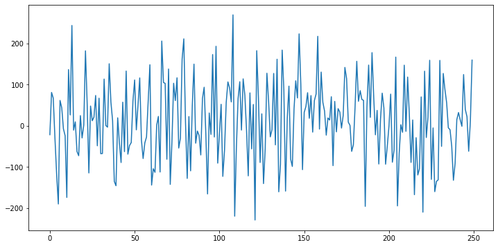

This time series is clearly random. The autocorrelation plot of this time series:

這個時間序列顯然是隨機的。 該時間序列的自相關圖：

from pandas.plotting import autocorrelation_plotplt.figure(figsize=(12,6))autocorrelation_plot(noise)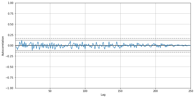

As expected, all autocorrelation values are very close to zero.

不出所料，所有自相關值都非常接近零。

Let’s do an example of non-random time series. The plot below shows a very simple upward trend.

讓我們舉一個非隨機時間序列的例子。 下圖顯示了非常簡單的上升趨勢。

upward = pd.Series(np.arange(100))upward.plot(figsize=(10,6))plt.grid()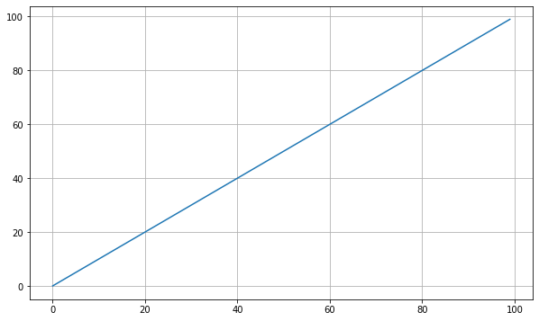

The autocorrelation plot for this time series:

此時間序列的自相關圖：

plt.figure(figsize=(12,6))autocorrelation_plot(upward)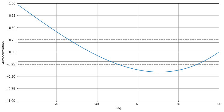

This autocorrelation clearly indicates a non-random time series as there are many significantly non-zero values.

由于存在許多明顯的非零值，因此這種自相關清楚地指示了非隨機時間序列。

It is very easy to visually check the non-randomness of simple upward and downward trends. However, in real life data sets, we are likely to see highly complex time series. We may not able see the trends or seasonality in those series. In such cases, autocorrelation plots are very helpful for time series analysis.

直觀地檢查簡單的向上和向下趨勢的非隨機性非常容易。 但是，在現實生活中的數據集中，我們可能會看到非常復雜的時間序列。 我們可能看不到那些系列的趨勢或季節性。 在這種情況下，自相關圖對于時間序列分析非常有幫助。

Pandas provide two more plotting tools which are bootstap plot and RadViz. They can also be used in exploratory data analysis process.

熊貓提供了另外兩種繪圖工具，即引導繪圖和RadViz 。 它們也可以用于探索性數據分析過程。

Thank you for reading. Please let me know if you have any feedback.

感謝您的閱讀。 如果您有任何反饋意見，請告訴我。