了解機器學習 (Understanding ML)

This article is based on my entry into DengAI competition on the DrivenData platform. I’ve managed to score within 0.2% (14/9069 as on 02 Jun 2020). Some of the ideas presented here are strictly designed for competitions like that and might not be useful IRL.

本文基于我 對DrivenData平臺上的DengAI競賽的參與 。 我的得分一直在0.2％以內(截至2020年6月2日，得分為14/9069)。 這里提出的一些想法是嚴格針對此類比賽而設計的，可能對IRL無效。

Before we start I have to warn you that some parts might be obvious for more advanced data engineers, and it’s a very long article. You might read it section by section of just pick the parts that are interesting for you:

在開始之前，我必須警告您，某些部分對于更高級的數據工程師可能是顯而易見的，并且這是一篇很長的文章。 您可能會逐節閱讀它，只是選擇一些您感興趣的部分：

DengAI, Data preprocessing

DengAI，數據預處理

More parts are coming soon…

更多零件即將推出…

問題描述 (Problem description)

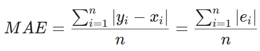
First, we need to discuss the competition itself. DengAI’s goal was (actually, at this moment even is, because the administration of DrivenData decided to make it “ongoing” competition, so you can join and try yourself) to predict a number of dengue cases in the particular week base on weather data and location. Each participant was given a training dataset and test dataset (not validation dataset). MAE ( Mean Absolute Error) is a metric used to calculate score and the training dataset covers 28 years of weekly values for 2 cities (1456 weeks). Test data is smaller and spans over 5 and 3 years (depends on the city).

首先，我們需要討論比賽本身。 DengAI的目標是(實際上，在此時此刻，甚至是因為DrivenData的管理部門決定使其正在進行的競爭，因此您可以加入并進行嘗試)根據天氣數據和位置。 每個參與者都得到了訓練數據集和測試數據集 (不是驗證數據集)。 MAE ( 平均絕對誤差 )是用于計算得分的指標，訓練數據集涵蓋2個城市(1456周)的28年每周值。 測試數據較小，跨度為5年和3年(取決于城市)。

For those who don’t know, Dengue fever is a mosquito-borne disease that occurs in tropical and sub-tropical parts of the world. Because it’s carried by mosquitoes, the transmission is related to climate and weather variables.

對于那些不知道的人，登革熱是一種蚊子傳播的疾病，發生在世界的熱帶和亞熱帶地區。 由于它是由蚊子攜帶的，因此傳播與氣候和天氣變量有關。

數據集 (Dataset)

If we look at the training dataset it has multiple features:

如果我們查看訓練數據集，它具有多種功能：

City and date indicators:

城市和日期指標：

• city — City abbreviations: sj for San Juan and iq for Iquitos

  city —城市縮寫： sj代表圣胡安， iq代表伊基托斯

• week_start_date — Date given in yyyy-mm-dd format

  week_start_date —以yyyy-mm-dd格式給出的日期

NOAA’s GHCN daily climate data weather station measurements:

NOAA的GHCN每日氣候數據氣象站測量結果：

• station_max_temp_c — Maximum temperature

  station_max_temp_c-最高溫度

• station_min_temp_c — Minimum temperature

  station_min_temp_c-最低溫度

• station_avg_temp_c — Average temperature

  station_avg_temp_c-平均溫度

• station_precip_mm — Total precipitation

  station_precip_mm —總降水量

• station_diur_temp_rng_c — Diurnal temperature range

  station_diur_temp_rng_c —晝夜溫度范圍

PERSIANN satellite precipitation measurements (0.25x0.25 degree scale):

PERSIANN衛星降水測量(0.25x0.25度標度)：

• precipitation_amt_mm — Total precipitation

  rainfall_amt_mm —總降水量

NOAA’s NCEP Climate Forecast System Reanalysis measurements (0.5x0.5 degree scale):

NOAA的NCEP氣候預測系統再分析測量結果(0.5x0.5度等級)：

• reanalysis_sat_precip_amt_mm — Total precipitation

  reanalysis_sat_precip_amt_mm —總降水量

• reanalysis_dew_point_temp_k — Mean dew point temperature

  reanalysis_dew_point_temp_k —平均露點溫度

• reanalysis_air_temp_k — Mean air temperature

  reanalysis_air_temp_k —平均氣溫

• reanalysis_relative_humidity_percent — Mean relative humidity

  reanalysis_relative_humidity_percent —平均相對濕度

• reanalysis_specific_humidity_g_per_kg — Mean specific humidity

  reanalysis_specific_humidity_g_per_kg —平均比濕度

• reanalysis_precip_amt_kg_per_m2 — Total precipitation

  reanalysis_precip_amt_kg_per_m2 —總降水量

• reanalysis_max_air_temp_k — Maximum air temperature

  reanalysis_max_air_temp_k —最高氣溫

• reanalysis_min_air_temp_k — Minimum air temperature

  reanalysis_min_air_temp_k —最低氣溫

• reanalysis_avg_temp_k — Average air temperature

  reanalysis_avg_temp_k —平均氣溫

• reanalysis_tdtr_k — Diurnal temperature range

  reanalysis_tdtr_k —日溫度范圍

Satellite vegetation — Normalized difference vegetation index (NDVI) — NOAA’s CDR Normalized Difference Vegetation Index (0.5x0.5 degree scale) measurements:

衛星植被-歸一化植被指數(NDVI)-NOAA的CDR歸一化植被指數(0.5x0.5度)：

• ndvi_se — Pixel southeast of city centroid

  ndvi_se —城市質心的東南像素

• ndvi_sw — Pixel southwest of city centroid

  ndvi_sw —城市質心的西南像素

• ndvi_ne — Pixel northeast of city centroid

  ndvi_ne —城市質心的東北像素

• ndvi_nw — Pixel northwest of city centroid

  ndvi_nw —城市質心的西北像素

Additionally, we have information about the number of total_cases each week.

此外，我們還提供有關每周total_cases數量的信息。

It is easy to spot that for each row in the dataset we have multiple features describing similar kinds of data. There are four categories:

很容易發現，對于數據集中的每一行，我們都有描述相似類型數據的多種功能。 有四個類別：

- temperature- precipitation- humidity- ndvi (those four features are referring to different points in the cities, so they are not exactly the same data)

-溫度-降水量-濕度-ndvi(這四個要素所指的是城市中的不同地點，因此它們并不是完全相同的數據)

Because of that, we should be able to remove some of the redundant data from the input. Ofc, we cannot just pick one temperature randomly. If we look at just temperature data there is a distinguishment between ranges (min, avg, max) and even type (mean dew point or diurnal).

因此，我們應該能夠從輸入中刪除一些冗余數據。 當然，我們不能隨便挑一個溫度。 如果僅查看溫度數據，則在范圍(最小值，平均值，最大值)和類型(平均露點或晝夜)之間存在區別。

輸入示例： (Input example:)

week_start_date 1994-05-07
total_cases 22
station_max_temp_c 33.3
station_avg_temp_c 27.7571428571
station_precip_mm 10.5
station_min_temp_c 22.8
station_diur_temp_rng_c 7.7
precipitation_amt_mm 68.0
reanalysis_sat_precip_amt_mm 68.0
reanalysis_dew_point_temp_k 295.235714286
reanalysis_air_temp_k 298.927142857
reanalysis_relative_humidity_percent 80.3528571429
reanalysis_specific_humidity_g_per_kg 16.6214285714
reanalysis_precip_amt_kg_per_m2 14.1
reanalysis_max_air_temp_k 301.1
reanalysis_min_air_temp_k 297.0
reanalysis_avg_temp_k 299.092857143
reanalysis_tdtr_k 2.67142857143
ndvi_location_1 0.1644143
ndvi_location_2 0.0652
ndvi_location_3 0.1321429
ndvi_location_4 0.08175

提交格式： (Submission format:)

city,year,weekofyear,total_cases
sj,1990,18,4
sj,1990,19,5
...

分數評估： (Score evaluation:)

數據分析 (Data Analysis)

Before even starting designing the models we need to look at the raw data and fix it. To accomplish that we’re going to use Pandas Library. Usually, we can just import .csv files out of the box and work on the imported DataFrame, but sometimes (especially when there is no column description in the first row) we have to provide a list of columns.

在甚至開始設計模型之前，我們需要查看原始數據并進行修復。 為此，我們將使用Pandas Library 。 通常，我們可以直接打開.csv文件并在導入的DataFrame上工作，但是有時(尤其是當第一行中沒有列說明時)，我們必須提供列列表。

import pandas as pd
pd.set_option("display.precision", 2)
df = pd.read_csv('./dengue_features_train_with_out.csv')
df.describe()

Pandas has a build-in method called describe which displays basic statistical info about columns in a dataset.

Pandas有一個稱為describe的內置方法，該方法顯示有關數據集中列的基本統計信息。

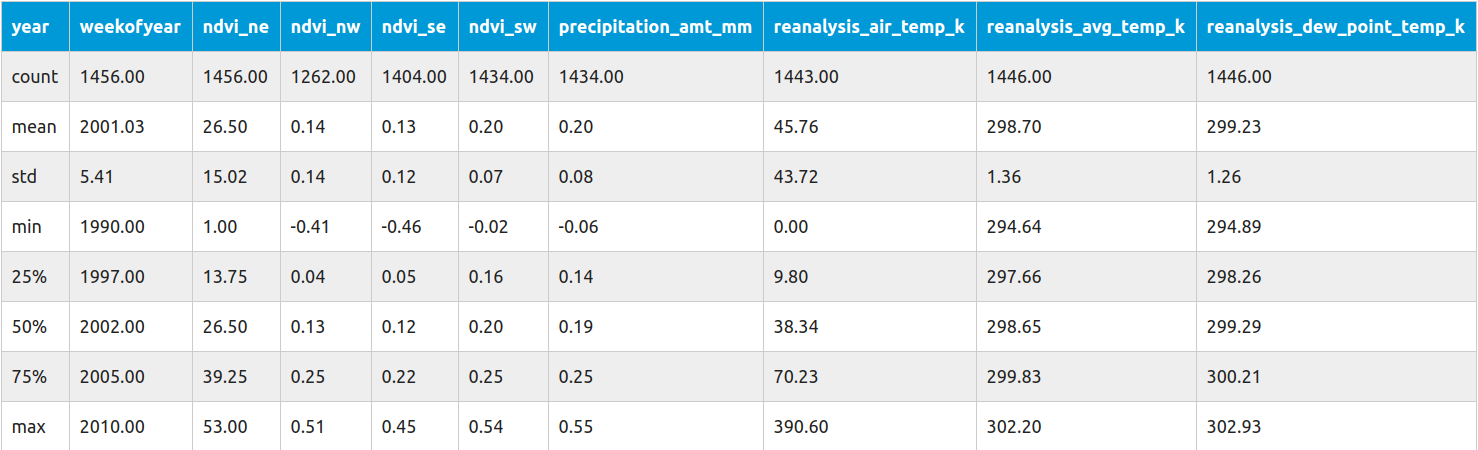
Naturally, this method works only on numerical data. If we have non-numerical columns we have to do some preprocessing first. In our case, the only column that is a categorical column is city. This column contains only two values sj and iq and we’re going to deal with it later.

自然，此方法僅適用于數值數據。 如果我們有非數字列，則必須先進行一些預處理。 在我們的例子中，唯一的列是city 。 該列僅包含兩個值sj和iq ，稍后我們將對其進行處理。

Back to the main table. Each row contains a different kind of information:

回到主表。 每行包含不同類型的信息：

• count — describes the number of non-NaN values, basically how many values are correct, not empty number

  count —描述非NaN值的數量，基本上是多少個正確的值，不是空值

• mean — mean value from the whole column (useful for normalization)

  平均值 -整列的平均值(用于歸一化)

• std — standard deviation (also useful for normalization)

  std-標準偏差(也可用于標準化)

• min -> max — shows us a range in which values are contained (useful for scaling)

  min- > max-向我們顯示一個包含值的范圍(用于縮放)

Let us start with the count. It is important to know how many records in your dataset has missing data (one or many) an decide what to do with them. If you look at the ndvi_nw value, it is empty in 13.3% of cases. That might be a problem if you decide to replace missing values with some arbitrary value like 0. Usually, there are two common solutions to this problem:

讓我們從伯爵開始。 重要的是要知道數據集中有多少記錄缺少數據(一個或多個)，并決定如何處理它們。 如果查看ndvi_nw值，則在13.3％的情況下該值為空。 如果您決定用某些任意值(例如0)替換缺失值，則可能會遇到問題。通常，有兩種常見的解決方案：

• set an average value

  設定平均值

• do the interpolation

  進行插值

Interpolation (dealing with missing data)

插值(處理丟失的數據)

When dealing with series data (like we do) it’s easier to interpolate (average from just the neighbors) value from its neighbors instead of replacing it with just an average from the entire set. Usually, series data have some correlation between values in the series, and using neighbors gives a better result. Let me give you an example.

在處理序列數據時(像我們一樣)，更容易從鄰居內插值(僅來自鄰居的平均值)，而不是僅用整個集中的平均值替換它。 通常，系列數據在系列中的值之間具有一定的相關性，使用鄰居可以得到更好的結果。 讓我舉一個例子。

Suppose you’re dealing with temperature data, and your entire dataset consists of the values from January to December. The average value from the entire year is going to be an invalid replacement for missing days throughout most of the year. If you take days from July then you might have values like [28, 27, -, -, 30] (or [82, 81, -, -, 86] for those who prefer imperial units). If that would be a London then an annual average temperature is 11C (or 52F). Using 11 seams wrong in this case, doesn’t it? That’s why we should use interpolation instead of the average. With interpolation (even in the case when there is a wider gap) we should be able to achieve a better result. If you calculate values you should get (27+30)/2=28.5 and (28.5+30)/2=29.25 so at the end our dataset will look like [28, 27, 28.5, 29.25, 30], way better than [28, 27, 11, 11, 30].

假設您要處理溫度數據，并且整個數據集都包含一月到十二月的值。 全年的平均值將替代一年中大部分時間的缺勤天數。 如果您從7月開始花費幾天的時間，則可能會使用[28，27，-，-，30]之類的值 (對于喜歡英制單位的人，則可能是[ 82，81，-，-，86] )。 如果那是倫敦，那么年平均氣溫為11攝氏度(或52華氏度)。 在這種情況下使用11個接縫是錯誤的，不是嗎？ 這就是為什么我們應該使用插值法而不是平均值法。 通過插值(即使在間隙更大的情況下)，我們也應該能夠獲得更好的結果。 如果您計算值，則應該得到(27 + 30)/2=28.5和(28.5 + 30)/2=29.25，所以最后我們的數據集看起來像[ 28，27，28.5，29.25，30 ] ，比[28、27、11、11、30] 。

Splitting dataset into cities

將數據集劃分為城市

Because we’ve already covered some important things lets define a method which allows us to redefine our categorical column ( city) into binary column vectors and interpolate data:

因為我們已經介紹了一些重要的事情，所以讓我們定義一個方法，該方法可以將分類列( city )重新定義為二進制列向量并插值數據：

def extract_data(train_file_path, columns, categorical_columns=CATEGORICAL_COLUMNS, categories_desc=CATEGORIES,
                 interpolate=True):
    # Read csv file and return
    all_data = pd.read_csv(train_file_path, usecols=columns)
    if categorical_columns is not None:
        # map categorical to columns
        for feature_name in categorical_columns:
            mapping_dict = {categories_desc[feature_name][i]: categories_desc[feature_name][i] for i in
                            range(0, len(categories_desc[feature_name]))}
            all_data[feature_name] = all_data[feature_name].map(mapping_dict)
        # Change mapped categorical data to 0/1 columns
        all_data = pd.get_dummies(all_data, prefix='', prefix_sep='')
    # fix missing data
    if interpolate:
        all_data = all_data.interpolate(method='linear', limit_direction='forward')
    return all_data

All constants (like CATEGORICAL_COLUMNS) are defined in this Gist.

所有常量(例如CATEGORICAL_COLUMNS)都在 此Gist 中定義 。

This function returns a dataset with two binary columns called sj and iq which are having true values where city was set to be either sj or iq.

此函數返回具有兩個名為sj和iq的二進制列的數據集，這些列具有真實值，其中city設置為sj或iq 。

繪制數據 (Plotting the data)

It is important to plot your data to get a visual understanding of how values are distributed in the series. We’re going to use a library called Seaborn to help us with plotting data.

重要的是繪制數據以直觀了解值在系列中的分布方式。 我們將使用一個名為Seaborn的庫來幫助我們繪制數據。

sns.pairplot(dataset[["precipitation_amt_mm", "reanalysis_sat_precip_amt_mm", "station_precip_mm"]], diag_kind="kde")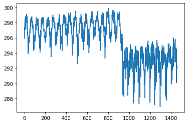

Here we have just one feature from the dataset, and we can clearly distinguish seasons and cities (the point when the average value drops from ~297K to ~292K).

在這里，我們僅從數據集中獲得一個特征，我們可以清楚地區分季節和城市(均值從?297K降至?292K)。

Another thing that could be useful is a pair correlation between different features. That way we could be able to remove some of the redundant features from our dataset.

可能有用的另一件事是不同功能之間的成對關聯 。 這樣，我們便可以從數據集中刪除一些冗余特征。

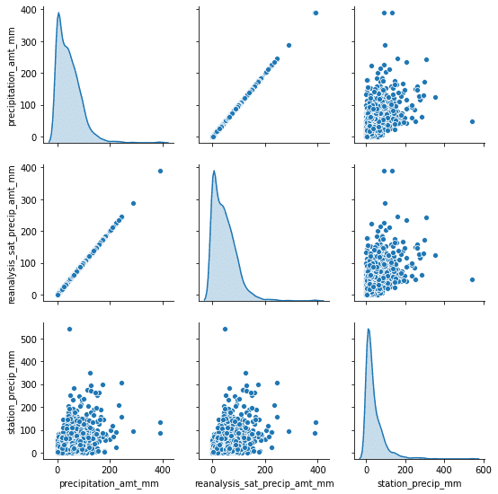
As you can notice, we can drop one of the precipitation features right away. It might be unintentional at first but because we have data from different sources, the same kind of data (like precipitation) won’t always be fully correlated with each other. This might be due to different measurement methods or something else.

如您所見，我們可以立即刪除其中一個降水特征。 乍一看可能不是故意的，但是由于我們有來自不同來源的數據，因此相同類型的數據(例如降水)將不會總是彼此完全相關。 這可能是由于不同的測量方法或其他原因造成的。

數據關聯 (Data Correlation)

When working with a lot of features we don’t really have to plot pair plots for every pair like that. Another option is just to calculate sth called Correlation Score. There are different types of correlations for a different types of data. Because our dataset consists only of numerical data we can use the builtin method called .corr() to generate correlations for each city.

當使用許多功能時，我們實際上不必像這樣為每對繪制圖。 另一種選擇是只計算某項，稱為Correlation Score 。 對于不同類型的數據，存在不同類型的關聯。 因為我們的數據集僅包含數字數據，所以我們可以使用稱為.corr()的內置方法為每個城市生成相關性。

If there are categorical columns which shouldn’t be treated as binary you could calculate Cramér’s V measure of association to find out a “correlation” between them and the rest of the data.

如果存在不應被視為二進制的分類列，則可以計算 Cramér的V關聯度量， 以找出它們與其余數據之間的“關聯”。

import pandas as pd
import seaborn as sns
# Importing our extraction function
from helpers import extract_data
from data_info import *
train_data = extract_data(train_file, CSV_COLUMNS)
# Get data for "sj" city and drop both binary columns
sj_train = train_data[train_data['sj'] == 1].drop(['sj', 'iq'], axis=1)
# Generate heatmap
corr = sj_train.corr()
mask = np.triu(np.ones_like(corr, dtype=np.bool))
plt.figure(figsize=(20, 10))
ax = sns.heatmap(
    corr, 
     mask=mask, 
    vmin=-1, vmax=1, center=0,
    cmap=sns.diverging_palette(20, 220, n=200),
    square=True
)
ax.set_title('Data correlation for city "sj"')
ax.set_xticklabels(
    ax.get_xticklabels(),
    rotation=45,
    horizontalalignment='right'
);

You could do the same for iq city and compare both of them (correlations are different).

您可以對iq city進行相同的操作，然后將它們進行比較(相關性不同)。

If you look at this heatmap it’s obvious which features are correlated with each other and which are not. You should be aware there are positive and negative correlations (dark blueish and dark red). Features without correlation are white. There are groups of positively correlated features and unsurprisingly they are referring to the same type of measurement (correlation between station_min_temp_c and station_avg_temp_c). But there are also correlations between different kind of features (like reanalysis_specific_humidity_g_per_kg and reanalysis_dew_point_temp_k). We should also focus on the correlation between total_cases and the rest of the features because that’s what we have to predict.

如果您查看此熱圖，很明顯哪些功能是相互關聯的，哪些功能是不相關的。 您應該知道，存在正相關和負相關(深藍色和深紅色)。 沒有關聯的要素是白色。 有成組的正相關特征，毫不奇怪，它們指的是同一類型的測量( station_min_temp_c和station_avg_temp_c之間的相關性)。 但是，不同類型的功能(例如reanalysis_specific_humidity_g_per_kg和reanalysis_dew_point_temp_k )之間也存在相關性。 我們還應該關注total_cases與其余功能之間的相關性，因為這是我們必須預測的。

This time we’re out of luck because nothing is really strongly correlated with our target. But we still should be able to pick the most important features for our model. Looking on the heatmap is not that useful right now so let me switch to the bar plot.

這次我們很不走運，因為沒有任何東西與我們的目標真正相關。 但是我們仍然應該能夠為模型選擇最重要的功能。 現在查看熱圖并不是那么有用，所以讓我切換到條形圖。

sorted_y = corr.sort_values(by='total_cases', axis=0).drop('total_cases')
plt.figure(figsize=(20, 10))
ax = sns.barplot(x=sorted_y.total_cases, y=sorted_y.index, color="b")
ax.set_title('Correlation with total_cases in "sj"')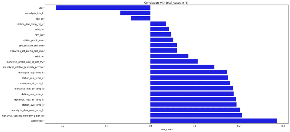

Usually, when picking features to our model we’re choosing features that have the highest absolute correlation value with our target. It’s up to you to decide how many features you choose, you might even choose all of them but that’s usually not the best idea.

通常，在為模型選擇要素時，我們會選擇與目標具有最高絕對相關值的要素。 由您決定選擇多少個功能，甚至可以選擇所有功能，但這通常不是最好的主意。

It is also important to look at how target values are distributed within our dataset. We can easily do that using pandas:

查看目標值在數據集中的分布方式也很重要。 我們可以使用熊貓輕松地做到這一點：

On an average number of cases for a week is quite low. Only from time to time (once a year), total number of cases jumps to some higher value. We need to remember that when designing our model because even if we manage to find that “jumps” we might lose a lot during the weeks with little or none cases.

平均而言，一周的病例數很低。 僅每隔一段時間(一年一次)，病例總數就會躍升至更高的水平。 我們需要記住，在設計模型時，因為即使我們設法找到“跳躍”，我們也可能在幾周內損失很少甚至沒有的情況下損失很多。

什么是NDVI值？ (What is an NDVI value?)

Last thing we have to discuss in this article in an NDVI index ( Normalized difference vegetation index). This index is an indicator of vegetation. High negative values correspond to water, values close to 0 represent rocks/sand/snow, and values close to 1 tropical forests. In the given dataset, we have 4 different NDVI values for each city (each for a different corner on the map).

我們在本文中最后要討論的是NDVI指數 ( 歸一化植被指數 )。 該指數是植被的指標。 高負值表示水，接近0的值表示巖石/沙地/雪，接近1的熱帶森林。 在給定的數據集中，每個城市有4個不同的NDVI值(每個都對應于地圖上的不同角)。

Even if the overall NDVI index is quite useful to understand a type of terrain we’re dealing with and if we would need to design a model for multiple cities that might come in handy, but in this case, we have only two cities which climate and position on the map are known. We don’t have to train our model to figure out which kind of environment we’re dealing with, instead, we can just train two separate models for each city.

即使總體NDVI指數對于了解我們正在處理的地形類型非常有用，并且我們需要為可能會派上用場的多個城市設計模型，但是在這種情況下，我們只有兩個城市和在地圖上的位置是已知的。 我們不必訓練模型就可以確定要處理的環境，相反，我們可以為每個城市訓練兩個??單獨的模型。

I’ve spent a while trying to make use of those values (especially that interpolation is hard in this case because we’re using a lot of information during the process). Using the NDVI index might be also misleading because changes in values don’t have to correspond to changes in the vegetation process.

我花了一段時間嘗試使用這些值(特別是在這種情況下很難插值，因為在此過程中我們使用了大量信息)。 使用NDVI指數也可能會產生誤導，因為值的變化不必與植被過程的變化相對應。

If you want to check those cities out pleas refer to San Juan, Puerto Rico, and Iquitos, Peru.

如果要檢查這些城市，請參閱波多黎各的San Juan和秘魯的Iquitos 。

結論 (Conclusion)

At this point, you should be aware of how our dataset looks like. We didn’t even start designing the first model but already know that some of the features are less important than others and some of them are just repeating the same data. If you would need to take with you one thing from this entire article, it is “Try to understand your data first!”.

此時，您應該了解我們的數據集的外觀。 我們甚至沒有開始設計第一個模型，但已經知道某些功能不如其他功能重要，而某些功能只是重復相同的數據。 如果您需要從整篇文章中帶走一件事，那就是“嘗試先了解您的數據！”。

Originally published at https://erdem.pl.

最初發布在 https://erdem.pl 。