Memory-Associated Differential Learning論文及代碼解讀

論文來源：

論文PDF：

Memory-Associated Differential Learning論文

論文代碼：

Memory-Associated Differential Learning代碼

論文解讀：

1.Abstract

Conventional Supervised Learning approaches focus on the mapping from input features to output labels. After training, the learnt models alone are adapted onto testing features to predict testing labels in isolation, with training data wasted and their associations ignored. To take full advantage of the vast number of training data and their associations, we propose a novel learning paradigm called Memory-Associated Differential (MAD) Learning. We first introduce an additional component called Memory to memorize all the training data. Then we learn the differences of labels as well as the associations of features in the combination of a differential equation and some sampling methods. Finally, in the evaluating phase, we predict unknown labels by inferencing from the memorized facts plus the learnt differences and associations in a geometrically meaningfull manner. We gently build this theory in unary situations and apply it on Image Recognition, then extend it into Link Prediction as a binary situation, in which our method outperforms strong state-of-the-art baselines on three citation networks and ogbl-ddi dataset.
傳統的監督學習方法側重于從輸入特征到輸出標簽的映射。 在訓練之后，單獨學習的模型被調整到測試特征上以單獨預測測試標簽，訓練數據被浪費并且它們的關聯被忽略。 為了充分利用大量的訓練數據及其關聯，我們提出了一種新的學習范式，稱為記憶關聯差分學習。 我們首先引入一個名為Memory的附加組件來記憶所有的訓練數據。 然后在微分方程和一些抽樣方法的組合中，我們學習標簽的差異以及特征的關聯。 最后，在評估階段，我們通過從記憶的事實加上學習的差異和聯系中推斷出幾何意義上的完全方式來預測未知標簽。 我們在一元情況下溫和地構建這一理論，并將其應用于圖像識別，然后將其擴展為二元情況下的鏈接預測，其中我們的方法在三個引用網絡和ogbl-ddi數據集上優于強大的最先進的基線。

2.Introduction

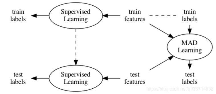
Figure 1: The difference between Conventional Supervised Learning and MAD Learning. The former learns the mapping from features to labels in training data and apply this mapping on testing data, while the latter learns the differences and associations among data and inferences testing labels from memorized training data.
圖1:常規監督學習和MAD學習的區別。 前者學習訓練數據中從特征到標簽的映射，并將該映射應用于測試數據，而后者學習數據之間的差異和關聯，并從記憶的訓練數據中推斷測試標簽。

3.Related Works

Instead of treating External Memory as a way to add more learnable parameters to store uninterpretable hidden states, we try to memorize the facts as they are, and then learn the differences and associations between them.
我們不是把外部記憶當作一種添加更多可學習的參數來存儲無法解釋的隱藏狀態的方式，而是試圖記住事實的本來面目，然后學習它們之間的區別和聯系。

Most of the experiments in this article are designed to solve Link Prediction problem that we predict whether a pair of nodes in a graph are likely to be connected, how much the weight their edge bares, or what attributes their edge should have.
本文中的大部分實驗都是為了解決鏈接預測問題，即我們預測圖中的一對節點是否可能連通，它們的邊露出多少權重，或者它們的邊應該具有什么屬性。

Although our method is derived from a different perspective of view, we point out that Matrix Factorization can be seen as a simplification of MAD Learning with no memory and no sampling.
雖然我們的方法是從不同的角度推導出來的，但我們指出，矩陣分解可以被視為無記憶、無采樣的MAD學習的簡化。

4.Proposed Approach

4.1 Memory-Associated Differential Learning

By applying Mean Value Theorem for Definite Integrals [Comenetz, 2002], we can estimate the unknown y with known y0 if x0 is close enough to x:
應用定積分中值定理[Comenetz，2002]，如果x0與x足夠接近，我們可以用已知y0來估計未知y:

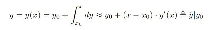
In such way, we connect the current prediction tasks y to the past fact y0, which can be stored in external memory, and convert the learning of our target function y(x) to the learning of a differential function y0(x), which in general is more accessible than the former.
以這種方式，我們將當前預測任務y連接到可以存儲在外部存儲器中的過去事實y0，并將我們的目標函數y(x)的學習轉換成微分函數y0(x)的學習，微分函數y0(x)通常比前者更容易訪問。

4.2 Inferencing from Multiple References

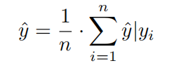
To get a steady and accurate estimation of y, we can sample n references x1, x2, · · · , xn to get n estimations y?|y1, y?|y2, · · · , y?|yn and combine them with an aggregator such as mean:
為了獲得對y的穩定而精確的估計，我們可以對n個參考x1、x2、、、xn進行采樣，以獲得n個估計yˇ| y1、yˇ| y2、，yˇ| yn，并將它們與均值結合。

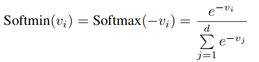
Here we adopt a function Softmin derived from Softmax which rescales the inputted d-dimentional array v so that every element of v lies in the range [0,1] and all of them sum to 1:
這里，我們采用從Softmax導出的函數Softmin，該函數對輸入的d維數組v進行重新縮放，使得v的每個元素都位于[0，1]的范圍內，并且它們的總和為1：

By applying Softmin we get the aggregated estimation:
通過Softmin最小，我們得到了總的估計:


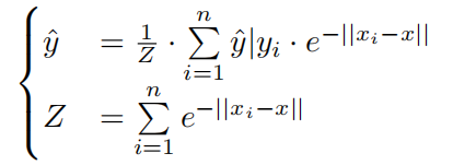
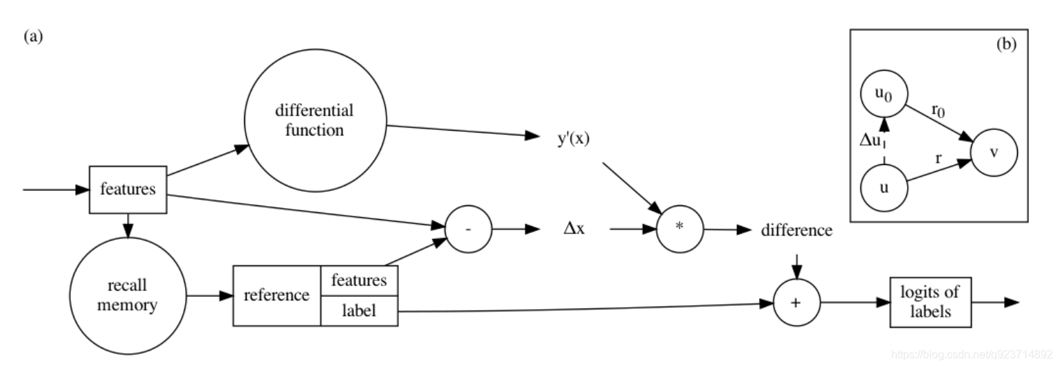
Figure 2: (a) Memory-Associated Differential Learning inferences labels from memorized ones following the first-order Taylor series approximation: y ≈ y0 +?x · y0(x). (b) In binary MAD Learning, when v = v0 holds, ?u?r |(u,v) is simplified to be ?u?r |v since it is the change
圖2: (a)記憶相關差分學習根據一階泰勒級數近似從記憶的標簽中推斷標簽:y≈y0+?x y0(x)。(b)在二進制MAD學習中，當v = v0成立時，?u?r |(u，v)簡化為?u?r |v，因為它是變化在v固定的情況下，將u輕微移動到u0后的r。

4.3 Soft Sentinels and Uncertainty

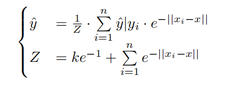
we introduce a mechanism on top of Softmin named Soft Sentinel. A Soft Sentinel is a dummy element mixed into the array of estimations with no information (e.g. the logit is 0) but a set distance (e.g. 0).
我們在Softmin之上引入了一個名為Soft Sentinel的機制。 軟哨點是一個混合到無信息估計數組中的虛擬元素(例如： logit為0)但是設定的距離(例如.：0).

The estimation after k Soft Sentinels distant at 1 added is：
增加k個軟哨兵距離為1后的估計值為：

When Soft Sentinels involved, only estimations given by close-enough references can have most of their impacts on the final result that unreliable estimations are supressed.
當涉及軟哨兵時，只有由足夠接近的參考文獻給出的估計才能對最終結果產生最大影響，即抑制不可靠的估計。

4.4 Other Details
For the sake of flexibility and performance, we usually do not use inputted features x directly, but to first convert x into position f(x).
為了靈活性和性能，我們通常不直接使用輸入的特征x，而是先將x轉換為位置f(x)。

To adapt to this situation, we generally wrap the memory with an adaptor function m such as a one-layer MLP, getting y?|y0 = m(y0) + (f(x) ? f(x0)) · g(x) where g(x) stands for gradient.
為了適應這種情況，我們通常用適配器函數m包裝存儲器，例如一層MLP，得到y\ | y0 = m(y0)+(f(x)-f(x0))g(x)，其中g(x)代表梯度。

When the encodings of nodes are dynamic and no features are provided, we usually adopt Random Mode in the training phase for efficiency and adopt Dynamic NN Mode in the evaluation phase for performance.
當節點的編碼是動態的并且沒有提供特征時，我們通常在訓練階段采用隨機模式來提高效率，在評估階段采用動態神經網絡模式來提高性能。

4.5 Binary MAD Learning
We model the relationship between a pair of nodes in a graph by extending MAD Learning into binary situations.
我們通過將MAD學習擴展到二元情況來建模圖中一對節點之間的關系。

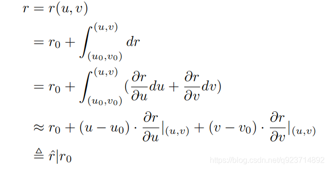
Therefore, we may further assume ?r?u |(u,v) = g1(v) if v = v0 and ?r?v |(u,v) = g2(u) if u = u0, making

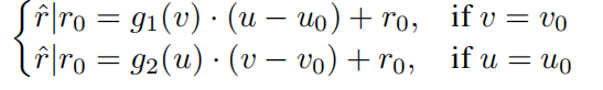
Here g1(·) is destination differential function and g2(·) is source differential function. If the edge is undirected, these two functions can be shared.
這里g1()是目的微分函數，g2()是源微分函數。 如果邊是無向的，這兩個函數可以共享。

5.Experiments

In the training phase, we sample arbitrary pairs of nodes to construct negative samples [Grover and Leskovec, 2016] and compare the scores between connected pairs and negative samples with Cross-Entropy as the loss function:
在訓練階段，我們對任意節點對進行采樣，構造負樣本[Grover和Leskovec，2016]，并以交叉熵為損失函數，比較連通對和負樣本之間的得分:

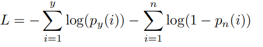
where y is the number of positive samples and n of negative samples, py(i) is the predicted probability of the i-th positive sample and pn(i) of the i-th negative sample. In the evaluating phase, we record the scores not only in Dynamic NN Mode but also in Random Mode.
其中y是正樣本的數量，n是負樣本的數量，py(i)是第I個正樣本的預測概率，pn(i)是第I個負樣本的預測概率。 在評估階段，我們不僅在動態神經網絡模式下記錄分數，還在隨機模式下記錄分數。

We have these three experimental settings to examine the contribution of Softmin and Soft Sentinels:

mean. Estimations are aggregated by mean function.
softmin. Estimations given by different references are summed up weighted by the results of Softmin applied to the distances.
sentinel. Estimations of softmin with 8 Soft Sentinels at distance 1 added.
As is shown in Figure 4(b), it is no much difference between mean and Softmin. But when mixed with Soft Sentinels, MAD Learning performs better and converges faster.
我們有這三個實驗設置來檢驗軟敏和軟哨兵的貢獻:
mean: 估計通過均值函數聚合。
softmin: 不同參考文獻給出的估計值通過應用于距離的軟最小結果進行加權求和。
sentinel:在距離1處增加了8個軟哨兵時，軟敏度的估計值。
如圖4(b)所示，平均值和軟最小值之間沒有太大差異。 但是當與軟哨兵混合時，MAD學習表現更好，收斂更快。

we repeat that MAD Learning does not predict directly. From another point of view, this experiment implies that undirect references can also be beneficial on par with direct information.
我們重申，MAD學習不能直接預測。 從另一個角度來看，這個實驗意味著無向引用與直接信息一樣有益。

6.Discussion

by extending it from a scalar to a vector, MAD Learning can be used for graphs with featured edges.
通過將它從標量擴展到向量，MAD學習可以用于具有特征邊的圖。

We also point out that MAD Learning can learn relations in heterogeneous graphs where nodes belong to different types (usually represented by encodings in different lengths). The only requirement is that positions of the source nodes should match with gradients of the destination nodes and vice versa.
我們還指出，MAD Learning可以學習節點屬于不同類型(通常由不同長度的編碼表示)的異構圖中的關系。 唯一的要求是源節點的位置應該與目標節點的梯度相匹配，反之亦然。

7. Conclusion

In this work, we explore a novel learning paradigm which is flexible, effective and interpretable. The outstanding results, especially on Link Prediction, open the door for several research directions:

1. The most important part of MAD Learning is memory.However, MAD Learning have to index the whole training data for random access. In Link Prediction, we implement memory as a dense adjacency matrix which results in huge occupation of space. The way to shrink memory and improve the utilization of space should be investigated in the future.

2. Based on memory as the ground-truth, MAD Learning appends some difference as the second part. We implement this difference simply as the product of distance and differential function, but we believe there exist different ways to model it.

3. The third part of MAD Learning is the similarity, which is used to assign weights to estimations given by different references. We reuse distance to compute the similarity, but decoupling it by some other embeddings and some other measurements such as inner product should also be worthy to explore.

4. In this work, we do deliberately not combine direct information to focus only on MAD Learning. Since MAD Learning takes another parallel route to predict, we believe integrating MAD Learning and Conventional Supervised Learning is also a promising direction.

在這項工作中，我們探索了一種靈活、有效和可解釋的新型學習范式。 突出的結果，尤其是在鏈接預測方面，為幾個研究方向打開了大門:

1. MAD學習最重要的部分是記憶.然而，MAD Learning必須對整個訓練數據進行索引，以便隨機訪問。 在鏈路預測中，我們將內存實現為密集的鄰接矩陣，這導致了巨大的空間占用。 未來應該研究縮小內存和提高空間利用率的方法。

2. 基于記憶作為基礎事實，MAD學習附加了一些區別作為第二部分。 我們將這種差異簡單地實現為距離和微分函數的乘積，但我們認為存在不同的建模方法。

3. MAD學習的第三部分是相似度，它被用來給不同參考文獻給出的估計賦值。 我們使用距離來計算相似度，但是通過一些其他嵌入和一些其他度量(例如內積)來解耦它也應該是值得探索的。

4. 在這項工作中，我們故意不結合直接信息，只專注于MAD學習。 由于MAD學習采取了另一種平行的預測路線，我們認為將MAD學習和常規監督學習相結合也是一個有前途的方向。

代碼解讀：

關于MAD函數主要參考了學長的文章Memory-Associated Differential Learning論文Link Prediction源碼解讀我太菜了=。=
主要是分析citations.py：

import torch
import torch.nn as nn
import torch.nn.functional as F
import torch.optim as optim
from torch.utils.data import DataLoader
import dgl
import dgl.nn
from sklearn import metrics#超參數
g_data_name = 'pubmed'  # cora | citeseer | pubmed
g_toy = False	#文中的涉及toy部分應該都屬于作者編寫代碼時的調試部分。
g_dim = 32  #對應論文中維度32維向量
n_samples = 8   #8個reference作為參考
total_epoch = 200
lr = 0.005
if g_toy:g_dim = g_dim // 2
elif g_data_name == 'pubmed':   #當對pubmed鏈接預測時，超參數的改變g_dim, n_samples, total_epoch, lr = 64, 64, 2000, 0.001def gpu(x):return x.cuda() if torch.cuda.is_available() else xdef cpu(x):return x.cpu() if torch.cuda.is_available() else xdef ip(x, y):return (x.unsqueeze(-2) @ y.unsqueeze(-1)).squeeze(-1).squeeze(-1)#unsqueeze(-2)在倒數第二個維度上增加一個維度，那么使用unsqueeze(-2)#squeeze(-1)在倒數第一維且該維維度為1時，去掉該維class MAD(nn.Module):def __init__(self, in_feats, n_nodes, node_feats,n_samples, mem, feats, gather2neighbor=False,):super(self.__class__, self).__init__()self.n_nodes = n_nodesself.node_feats = node_featsself.n_samples = n_samplesself.mem = memself.feats = featsself.gather2neighbor = gather2neighborself.f = gpu(nn.Linear(in_feats, node_feats))self.g = (None if gather2neighbor else gpu(nn.Linear(in_feats, node_feats)))# self.g相當于論文中的g(u)和g(v)中的g(x)函數，g(u)是r(u,v)在v_0處關于u的偏導數。# g(u)可以看作是當v=v_0時（把v當作是固定的），在r(u_0,v_0)的基礎上，# 將節點u移動到u_0（移動的距離很小，和微積分一個意思）后得到的r(u,v)的細微變化self.adapt = gpu(nn.Linear(1, 1))self.nn = Nonedef nns(self, src, dst):    #調試代碼if self.nn is None:n = self.n_samplesself.nn = gpu(torch.empty((self.n_nodes, n), dtype=int))for perm in DataLoader(range(self.n_nodes), 64, shuffle=False):self.nn[perm] = (self.feats[perm].unsqueeze(1) - self.feats.unsqueeze(0)).norm(dim=-1).topk(1 + n, largest=False).indices[..., 1:]return self.nn[src], self.nn[dst]def recall(self, src, dst):# 這里被調用是因為forward方法中調用了self.recall(mid0, dst.unsqueeze(1))# 所以，src=mid0，dst=dst.unsqueeze(1)# src的shape,是(1024,8)，dst的shape是(1024,1)# self.mem[src, dst]中mem是矩陣張量，src和dst也是矩陣張量，其實這里是觸發了廣播機制，# dst每一行的元素會和src每一行的元素兩兩組合成一個二維坐標來確定取mem中的哪一行哪一列的值，# 而mem因為是訓練集的鄰接矩陣，所以self.mem[src, dst]相當于是取1024×8個r_0# dst每一行的元素（1個）會和src每一行的8個元素進行組合，從而得到8個二維坐標。# 一對多，這就是python的廣播機制if self.mem is None:return 0return self.adapt((0.0 + self.mem[src, dst]).unsqueeze(-1)).squeeze(-1)# self.mem原來是bool型矩陣張量，(0.0 + self.mem[src, dst])使其變為數值型矩陣張量。# 目前來說，(0.0 + self.mem[src, dst])已經是取得的1024×8個r_0的數值形式，# 至于為什么要用self.adapt（定義為gpu(nn.Linear(1, 1))）進行線性變化，論文沒提，# 看來是沒有直接使用r_0(u_0,v_0),而是給每個r_0加了個可訓練的權重系數def forward(self, src, dst):# 該方法被mad(train_src[perm], train_dst[perm])這一句所調用，所以，src=train_src[perm]，dst=train_dst[perm]n = src.shape[0]#獲得邊的數目feats = self.feats#獲得節點特征g = self.f if self.gather2neighbor else self.g#如果有gather2neighbor（臨近值）則g=.f，否則g=.gmid0 = torch.randint(0, self.n_nodes, (n, self.n_samples))#生成的mid0 是形狀為n×self.n_samples的二維張量，數值是(0, self.n_nodes)mid1 = torch.randint(0, self.n_nodes, (n, self.n_samples))# mid0, mid1 = self.nns(src, dst)srcdiff = self.f(feats[src]).unsqueeze(1) - self.f(feats[mid0])# feats[src]的形狀是len(src)×節點特征維度，具體來說就是(1024,1433)，# self.f是__init__方法中定的線性變化，經過線性變化，# self.f(feats[src])的shape=(1024,32)# 由于mid0的shape=(1024,8)，所以feats[mid0]的shape=（1024,8,1433），# self.f(feats[mid0])的shape=（1024,8,32）。# feats[src]是該批次中所有邊的起始節點的特征，每個起始節點都要和8個reference節點# （因為self.n_samples=8）進行差分，從而實現論文3.5節中的(u-u_0)，這里有1024×8個u_0.# 對self.f(feats[src])使用unsqueeze(1)是為了將其shape變為(1024,1,32)，這樣# self.f(feats[src]).unsqueeze(1) - self.f(feats[mid0])就能自動觸發廣播機制，使得# 每條邊的起始節點的特征都能和8個reference節點的特征進行相減（差分），# 得到的srcdiff 的shape=（1024,8,32）logits1 = (ip(srcdiff, g(feats[dst]).unsqueeze(1))+ self.recall(mid0, dst.unsqueeze(1)))# logits1 這一步完成的是論文中的g(v)·(u-u_0)+r_0,when v=v_0，# 不過實現起來是按批進行處理，每一批1024條邊，每條邊有8個g(v)·(u-u_0)+r_0# 其中u和v都是一維向量，分別表示一條邊的起始節點和終點節點的特征# 具體分析如下：# 這里的ip()方法用于實現批量的g(v)·(u-u_0)操作（論文3.5節Link Prediction部分），# srcdiff是1024×8個(u-u_0)，# g(feats[dst]).unsqueeze(1)是該批次所有的g(v)，一共1024個，# g(feats[dst])的shape=(1024,32)，之所以要使用unsqueeze(1)使其shape變為(1024,1,32)# 是考慮到srcdiff 的shape=（1024,8,32），為了觸發廣播機制，# 使得每個g(v)都能和8個(u-u_0)進行操作（操作在ip方法中執行）# def ip(x, y):# return (x.unsqueeze(-2) @ y.unsqueeze(-1)).squeeze(-1).squeeze(-1)# 這里的x=srcdiff ，y=g(feats[dst]).unsqueeze(1)，x和y的形狀傳經過unsqueeze()變換以后# 分別變成了(1024,8,1,32)和(1024,1,32,1)，調用x@y進行矩陣乘法，# 實際是x和y的最里層的兩個維度# 進行矩陣乘法，即（1,32）×(32,1)=(1,1)，# 其物理意義為g(v)和(u-u_0)這兩個向量逐元素相乘并求和。# 最終得到的形狀是(1024,8,1,1)，然后經過squeeze(-1).squeeze(-1)后變為(1024,8)。# 至于self.recall(mid0, dst.unsqueeze(1))，# mid0的shape,是(1024,8)，dst.unsqueeze(1)的shape是(1024,1)，詳細分析見self.recall方法# recall方法返回的是論文中的1024×8個r_0(u_0,v_0)，1024是batch大小，# 8是每條邊的reference數量# ip()方法用于實現批量的g(v)·(u-u_0)，recall方法用于返回批量的r_0(u_0,v_0)，# 由此就完成了論文中的g(v)·(u-u_0)+r_0,when v=v_0dstdiff = self.f(feats[dst]).unsqueeze(1) - self.f(feats[mid1])# feats[dst]是該批次中所有邊的終點節點的特征，每個終點節點都要和8個reference節點# （因為self.n_samples=8）進行差分，從而實現論文3.5節中(v-v_0)，這里有8個v_0.logits2 = (ip(dstdiff, g(feats[src]).unsqueeze(1))+ self.recall(src.unsqueeze(1), mid1))# logits2 這一步完成的是論文中的8個g(u)·(v-v_0)+r_0,when u=u_0，logits = torch.cat((logits1, logits2), dim=1)dist = torch.cat((srcdiff, dstdiff), dim=1).norm(dim=2)# 這一步中，srcdiff和dstdiff的shape都是（1024,8,32），所以torch.cat((srcdiff, dstdiff), dim=1)# 得到的shape是（1024,16,32），使用norm(dim=2)是為了計算論文中的距離，（norm：求指定維度上的范數。）# 即在維度2上計算2范數，因為norm方法的參數p沒有指定，默認是計算2范數# 因此得到的dist的shape為（1024,16)logits = torch.cat((logits, gpu(torch.zeros(n, self.n_samples))), dim=1)# 使用8個 Soft Sentinels distant at 1，每個Soft Sentinel的logit是0，所以是使用zerosdist = torch.cat((dist, gpu(torch.ones(n, self.n_samples))), dim=1)# 每個Soft Sentinel的distance是1，所以是使用onesreturn torch.sigmoid(ip(logits, torch.softmax(-dist, dim=1)))dataset = (dgl.data.CoraGraphDataset() if g_data_name == 'cora'else dgl.data.CiteseerGraphDataset() if g_data_name == 'citeseer'else dgl.data.PubmedGraphDataset())#使用DGL提供的數據集，DGL官網有提供數據集的使用教程，網址：https://docs.dgl.ai/tutorials/blitz/2_dglgraph.html
graph = dataset[0]
#直接取出第一個graph
src, dst = graph.edges()
#獲取圖的所有邊，分別是起，終節點的編號序列
node_features = gpu(graph.ndata['feat'])
#獲取節點特征
node_labels = gpu(graph.ndata['label'])
#獲取節點標簽
train_mask = graph.ndata['train_mask']
#獲取決定節點是否屬于訓練集的一維掩碼張量，長度為graph中節點的數量，值為True表示對應的節點屬于訓練集
valid_mask = graph.ndata['val_mask']
#獲取決定節點是否屬于驗證集的一維掩碼張量
test_mask = graph.ndata['test_mask']
#獲取決定節點是否屬于測試集的一維掩碼張量
n_nodes = graph.num_nodes()
#獲取節點的數量
n_features = node_features.shape[1]
#shape[1]：表示矩陣的列數
#獲取節點的特征的維度
n_labels = int(node_labels.max().item() + 1)
#item()的作用是取出單元素張量的元素值并返回該值，保持該元素類型不變。
#獲取節點標簽的種類數量（通過最大標簽值+1獲得）adj = gpu(torch.zeros((n_nodes, n_nodes), dtype=bool))
adj[src, dst] = 1
adj[dst, src] = 1
#構建一個全0的鄰接矩陣矩陣，將邊輸入進去并對稱化
if g_toy:   #當toy模式采用全部的圖，應該是作者用來測試的部分mem = Nonetrain_src = gpu(src)train_dst = gpu(dst)mlp = gpu(nn.Linear(g_dim, n_labels))params = list(mlp.parameters())print('mlp params:', sum(p.numel() for p in params))mlp_opt = optim.Adam(params, lr=lr)
else:n = src.shape[0]#shape[0]就是讀取矩陣第一維度的長度，即讀取有多少條邊perm = torch.randperm(n)#隨機打亂n的序列val_num = int(0.05 * n) #劃分驗證集數量test_num = int(0.1 * n) #劃分測試集數量train_src = gpu(src[perm[val_num + test_num:]])train_dst = gpu(dst[perm[val_num + test_num:]])#訓練集是去掉驗證集和測試集剩下的部分val_src = gpu(src[perm[:val_num]])val_dst = gpu(dst[perm[:val_num]])#劃分驗證集test_src = gpu(src[perm[val_num:val_num + test_num]])test_dst = gpu(dst[perm[val_num:val_num + test_num]])#劃分測試集train_src, train_dst = (torch.cat((train_src, train_dst)),torch.cat((train_dst, train_src)))#torch.cat是將兩個張量（tensor）拼接在一起val_src, val_dst = (torch.cat((val_src, val_dst)),torch.cat((val_dst, val_src)))test_src, test_dst = (torch.cat((test_src, test_dst)),torch.cat((test_dst, test_src)))mem = gpu(torch.zeros((n_nodes, n_nodes), dtype=bool))mem[train_src, train_dst] = 1#獲得訓練集鄰接矩陣并且對稱化total_aucs = []
total_aps = []
for run in range(10):torch.manual_seed(run)  #設置隨機種子mad = MAD(  #調用MAD函數in_feats=n_features,n_nodes=n_nodes,node_feats=g_dim,n_samples=n_samples,mem=mem,feats=node_features,gather2neighbor=g_toy,)params = list(mad.parameters())print('params:', sum(p.numel() for p in params))#list（）將元組轉換為列表#構建好神經網絡后，網絡的參數都保存在parameters()函數當中，打印神經網絡結構opt = optim.Adam(params, lr=0.01)   #選擇Adam優化器best_aucs = [0, 0]best_aps = [0, 0]best_accs = [0, 0]for epoch in range(1, total_epoch + 1):mad.train() #將mad轉換到可訓練狀態for perm in DataLoader(range(train_src.shape[0]), batch_size=1024, shuffle=True):#range() 函數返回的是一個可迭代對象（類型是對象）#隨機打亂訓練節點數值序列,每1024為一組opt.zero_grad() #清空前一個epoch 殘留的梯度p_pos = mad(train_src[perm], train_dst[perm])#調用MAD中forward函數neg_src = gpu(torch.randint(0, n_nodes, (perm.shape[0], )))#random.randint()隨機生一個整數int類型，可以指定這個整數的范圍，同樣有上限和下限值#隨機生成作為負樣本的邊的起始節點和終點節點(創造負樣本)neg_dst = gpu(torch.randint(0, n_nodes, (perm.shape[0], )))idx = ~(mem[neg_src, neg_dst])#~是取反操作符#隨機生成的負樣本邊可能是正樣本邊，所以要提出這部分的負樣本邊，若原先是正樣本的邊也是負樣本，變為0p_neg = mad(neg_src[idx], neg_dst[idx])loss = (-torch.log(1e-5 + 1 - p_neg).mean()- torch.log(1e-5 + p_pos).mean())loss.backward()opt.step()if epoch % 10:continueif g_toy:with torch.no_grad():embed = mad.f(node_features)for i in range(100):mlp.train()mlp_opt.zero_grad()logits = mlp(embed)loss = F.cross_entropy(logits[train_mask], node_labels[train_mask])loss.backward()mlp_opt.step()with torch.no_grad():logits = mlp(embed)_, indices = torch.max(logits[valid_mask], dim=1)labels = node_labels[valid_mask]v_acc = torch.sum(indices == labels).item() * 1.0 / len(labels)_, indices = torch.max(logits[test_mask], dim=1)labels = node_labels[test_mask]t_acc = torch.sum(indices == labels).item() * 1.0 / len(labels)if v_acc > best_accs[0]:best_accs = [v_acc, t_acc]print(epoch, 'acc:', v_acc, t_acc)continuewith torch.no_grad():mad.eval()aucs = []aps = []for src, dst in ((val_src, val_dst), (test_src, test_dst)):p_pos = mad(src, dst)n = src.shape[0]perm = torch.randperm(n * 2)neg_src = torch.cat((src, gpu(torch.randint(0, n_nodes, (n, )))))[perm]neg_dst = torch.cat((gpu(torch.randint(0, n_nodes, (n, ))), dst))[perm]idx = ~(adj[neg_src, neg_dst])neg_src = neg_src[idx][:n]neg_dst = neg_dst[idx][:n]p_neg = mad(neg_src, neg_dst)y_true = cpu(torch.cat((p_pos * 0 + 1, p_neg * 0)))y_score = cpu(torch.cat((p_pos, p_neg)))fpr, tpr, _ = metrics.roc_curve(y_true, y_score, pos_label=1)#roc曲線繪制：#fpr：數組，隨閾值上漲的假陽性率#tpr：數組，隨閾值上漲的真正例率auc = metrics.auc(fpr, tpr)ap = metrics.average_precision_score(y_true, y_score)aucs.append(auc)aps.append(ap)if aucs[0] > best_aucs[0]:best_aucs = aucsprint(epoch, 'auc:', aucs)if aps[0] > best_aps[0]:best_aps = apsprint(epoch, 'ap:', aps)print(run, 'best auc:', best_aucs)print(run, 'best ap:', best_aucs)print(run, 'best acc (toy):', best_accs)total_aucs.append(best_aucs[1])total_aps.append(best_aps[1])
total_aucs = torch.tensor(total_aucs)
total_aps = torch.tensor(total_aps)
print('auc mean:', total_aucs.mean().item(), 'std:', total_aucs.std().item())
print('ap mean:', total_aps.mean().item(), 'std:', total_aps.std().item())

最后補上學長對MAD函數最后一個語句的分析，我確實想不到啊~