Logistic regression

數據內容： 兩個參數 x1 x2 y值 0 或 1

Potting

def read_file(file):data = pd.read_csv(file, names=['exam1', 'exam2', 'admitted'])data = np.array(data)return datadef plot_data(X, y):plt.figure(figsize=(6, 4), dpi=150)X1 = X[y == 1, :]X2 = X[y == 0, :]plt.plot(X1[:, 0], X1[:, 1], 'yo')plt.plot(X2[:, 0], X2[:, 1], 'k+')plt.xlabel('Exam1 score')plt.ylabel('Exam2 score')plt.legend(['Admitted', 'Not admitted'], loc='upper right')plt.show()print('Plotting data with + indicating (y = 1) examples and o indicating (y = 0) examples.')
plot_data(X, y)

從圖上可以看出admitted 和 not admitted 存在一個明顯邊界，下面進行邏輯回歸:
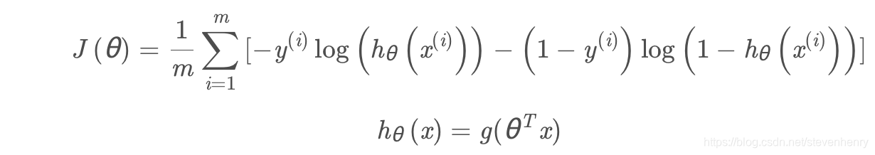
logistic 回歸的假設函數

g(x)為logistics function：

def sigmoid(x):return 1 / (np.exp(-x) + 1)

看一下邏輯函數的函數圖：

cost function
邏輯回歸的代價函數：

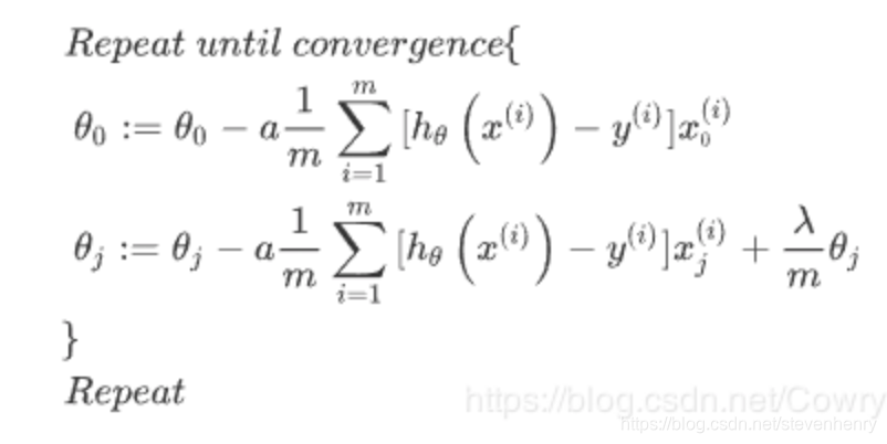
Gradient descent

• 批處理梯度下降（batch gradient descent）
• 向量化計算公式：
  $$1/m{X}^T(sigmoid(X{\theta }^T)?y)$$

def gradient(initial_theta, X, y):m, n = X.shapeinitial_theta = initial_theta.reshape((n, 1))grad = X.T.dot(sigmoid(X.dot(initial_theta)) - y) / mreturn grad.flatten()

computer Cost and grad

m, n = X.shape
X = np.c_[np.ones(m), X]
initial_theta = np.zeros((n + 1, 1))
y = y.reshape((m, 1))# cost, grad = costFunction(initial_theta, X, y)
cost, grad = cost_function(initial_theta, X, y), gradient(initial_theta, X, y)
print('Cost at initial theta (zeros): %f' % cost);
print('Expected cost (approx): 0.693');
print('Gradient at initial theta (zeros): ');
print('%f %f %f' % (grad[0], grad[1], grad[2]))
print('Expected gradients (approx): -0.1000 -12.0092 -11.2628')
#
theta1 = np.array([[-24], [0.2], [0.2]], dtype='float64')
cost, grad = cost_function(theta1, X, y), gradient(theta1, X, y)
# cost, grad = costFunction(theta1, X, y)
print('Cost at initial theta (zeros): %f' % cost);
print('Expected cost (approx): 0.218');
print('Gradient at initial theta (zeros): ');
print('%f %f %f' % (grad[0], grad[1], grad[2]))
print('Expected gradients (approx): 0.043 2.566 2.647')

學習 θ 參數
使用scipy庫里的optimize庫進行訓練， 得到最終的theta結果
Optimizing using fminunc

initial_theta = np.zeros(n + 1)
result = opt.minimize(fun=cost_function, x0=initial_theta, args=(X, y), method='SLSQP', jac=gradient)print('Cost at theta found by fminunc: %f' % result['fun'])
print('Expected cost (approx): 0.203')
print('theta:')
print('%f %f %f' % (result['x'][0], result['x'][1], result['x'][2]))
print('Expected theta (approx):')
print(' -25.161 0.206 0.201')

predict and Accuracies
學習好了參數θ， 開始進行預測， 當hθ 大于等于0.5， 預測y = 1
當hθ小于0.5時， 預測y =0

def predict(theta, X):m = np.size(theta, 0)rst = sigmoid(X.dot(theta.reshape(m, 1)))rst = rst > 0.5return rst# predict and Accuraciesprob = sigmoid(np.array([1, 45, 85], dtype='float64').dot(result['x']))
print('For a student with scores 45 and 85, we predict an admission ' \'probability of %.3f' % prob)
print('Expected value: 0.775 +/- 0.002\n')p = predict(result['x'], X)print('Train Accuracy: %.1f%%' % (np.mean(p == y) * 100))
print('Expected accuracy (approx): 89.0%\n')

也可以用skearn 來檢驗：

from sklearn.metrics import classification_report
print(classification_report(predictions, y))

Decision boundary (決策邊界)

X × θ = 0

θ0 + x1θ1 + x2θ2 = 0

x1 = np.arange(70, step=0.1)
x2 = -(final_theta[0] + x1*final_theta[1]) / final_theta[2]fig, ax = plt.subplots(figsize=(8,5))
positive = X[y == 1, :]
negative = X[y == 0, :]
ax.scatter(positive[:, 0], positive[:, 1], c='b', label='Admitted')
ax.scatter(negative[:, 0], negative[:, 1], s=50, c='r', marker='x', label='Not Admitted')
ax.plot(x1, x2)
ax.set_xlim(30, 100)
ax.set_ylim(30, 100)
ax.set_xlabel('x1')
ax.set_ylabel('x2')
ax.set_title('Decision Boundary')
plt.show()

Regularized logistic regression

正則化可以減少過擬合， 也就是高方差，直觀原理是，當超參數lambda 非常大的時候，參數θ相對較小， 所以函數曲線就變得簡單， 也就減少了剛方差。
可視化數據

data2 = pd.read_csv('ex2data2.txt', names=[' column1', 'column2', 'Accepted'])
data2.head()

def plot_data():positive = data2[data2['Accepted'].isin([1])]negative = data2[data2['Accepted'].isin([0])]fig, ax = plt.subplots(figsize=(8,5))ax.scatter(positive['column1'], positive['column2'], s=50, c='b', marker='o', label='Accepted')ax.scatter(negative['column1'], negative['column2'], s=50, c='r', marker='x', label='Rejected')ax.legend()ax.set_xlabel('Test 1 Score')ax.set_ylabel('Test 2 Score')plot_data()	

Feature mapping

盡可能將兩個特征 x1 x2 相結合，組成一個線性表達式，方法是映射到所有的x1 和x2 的多項式上，直到第六次冪

for i in 0..powerfor p in 0..i:output x1^(i-p) * x2^p```

def feature_mapping(x1, x2, power):data = {}for i in np.arange(power + 1):for p in np.arange(i + 1):data["f{}{}".format(i - p, p)] = np.power(x1, i - p) * np.power(x2, p)return pd.DataFrame(data)

Regularized Cost function

Regularized gradient decent

決策邊界
X × θ = 0

x = np.linspace(-1, 1.5, 250)
xx, yy = np.meshgrid(x, x)z = feature_mapping(xx.ravel(), yy.ravel(), 6).as_matrix()
z = z.dot(final_theta)
z = z.reshape(xx.shape)plot_data()
plt.contour(xx, yy, z, 0)
plt.ylim(-.8, 1.2)