本次練習的任務是使用邏輯歸回和神經網絡進行識別手寫數字(form 0 to 9, 自動手寫數字問題已經應用非常廣泛,比如郵編識別。
使用邏輯回歸進行多分類分類
練習2 中的logistic 回歸實現了二分類分類問題,現在將進行多分類,one vs all。
加載數據集
這次數據時MATLAB 的格式,使用Scipy.io.loadmat 進行加載。Scipy是一個用于數學、科學、工程領域的常用軟件包,可以處理插值、積分、優化、圖像處理、常微分方程數值解的求解、信號處理等問題。它可用于計算Numpy矩陣,使Numpy和Scipy協同工作。
import numpy as np
import scipy.io
from scipy.io import loadmat
import matplotlib.pyplot as plt
import scipy.optimize as optdata = scipy.io.loadmat('ex3data1.mat')
X = data['X']
y = data['y']

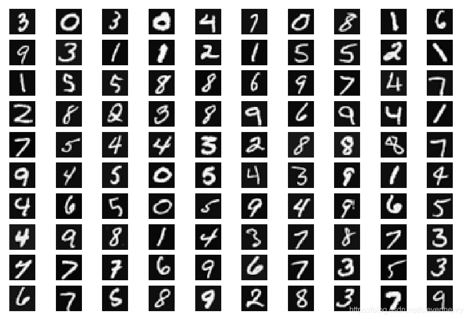
數據集共有5000個樣本, 每個樣本是20*20的灰度圖像。
visuazing the data
隨機展示100個圖像
def display_data(sample_images):fig, ax_array = plt.subplots(nrows=10, ncols=10, figsize=(6, 4))for row in range(10):for column in range(10):ax_array[row, column].matshow(sample_images[10 * row + column].reshape((20, 20)).T, cmap='gray')ax_array[row, column].axis('off')plt.show()returnrand_samples = np.random.permutation(X.shape[0]) # 打亂順序
sample_images = X[rand_samples[0:100], :]
display_data(sample_images)
Vectorizing Logistic Regression
看一下logistic回歸的代價函數:

其中:
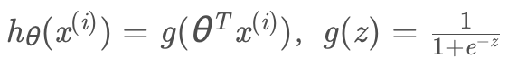
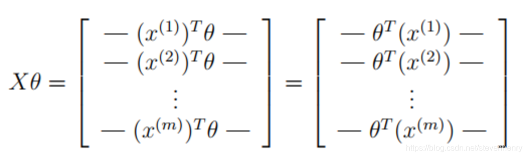
進行向量化運算:
def sigmoid(z):return 1 / (1 + np.exp(-z))
def regularized_cost(theta, X, y, l):thetaReg = theta[1:]first = (-y*np.log(sigmoid(X.dot(theta)))) + (y-1)*np.log(1-sigmoid(X.dot(theta)))reg = (thetaReg.dot(thetaReg))*l / (2*len(X))return np.mean(first) + reg
gradient
def regularized_gradient(theta, X, y, l):thetaReg = theta[1:]first = (1 / len(X)) * X.T @ (sigmoid(X.dot(theta)) - y)reg = np.concatenate([np.array([0]), (l / len(X)) * thetaReg])return first + reg
one-vs-all Classification
這個任務,有10個類,logistics是二分類算法,用在多分類上原理就是把所有的數據分為“某類”和“其它類”
from scipy.optimize import minimizedef one_vs_all(X, y, l, K):all_theta = np.zeros((K, X.shape[1])) # (10, 401)for i in range(1, K+1):theta = np.zeros(X.shape[1])y_i = np.array([1 if label == i else 0 for label in y])ret = minimize(fun=regularized_cost, x0=theta, args=(X, y_i, l), method='TNC',jac=regularized_gradient, options={'disp': True})all_theta[i-1,:] = ret.x return all_theta
向量化操作檢錯,經驗的機器學習工程師通常會檢驗矩陣的維度,來確認操作是否正確。
predict
def predict_one_vs_all(all_theta, X):m = np.size(X, 0)# You need to return the following variables correctly# Add ones to the X data matrixX = np.c_[np.ones((m, 1)), X]hypothesis = sigmoid(X.dot(all_theta.T)pred = np.argmax(hypothesis), 1) + 1return pred
這里的hypothesis.shape =[5000 * 10], 對應5000個樣本,每個樣本對應10個標簽的概率。取 概率最大的的值,作為最終預測結果。pred 是最終的5000個樣本預測數組。
pred = predict_one_vs_all(all_theta, X)
print('Training Set Accuracy: %.2f%%' % (np.mean(pred == y) * 100))
Neural Networks
這里只需要驗證所給權重數據,也就是theta,查看分類準確性。
## ================ Part 2: Loading Pameters ================
print('Loading Saved Neural Network Parameters ...')# Load the weights into variables Theta1 and Theta2
weight = scipy.io.loadmat('ex3weights.mat')
Theta1, Theta2 = weight['Theta1'], weight['Theta2']
predict
def load_weight(path):data = loadmat(path)return data['Theta1'], data['Theta2']theta1, theta2 = load_weight('ex3weights.mat')
theta1.shape, theta2.shapeX = np.insert(X, 0, values=np.ones(X.shape[0]), axis=1)  # intercept
#
#正向傳播
a1 = X
z2 = a1.dot(theta1.T)
z2.shape
z2 = np.insert(z2, 0, 1, axis=1)
a2 = sigmoid(z2)
a2.shape
z3 = a2.dot(theta2.T)
z3.shape
a3 = sigmoid(z3)
a3.shapey_pred = np.argmax(a3, axis=1) + 1
accuracy = np.mean(y_pred == y)
print ('accuracy = {0}%'.format(accuracy * 100)) # accuracy = 97.52%


)


)


