As the title states this is the last project from Udacity Nanodegree. The goal of this project is to analyze demographics data for customers of a mail-order sales company in Germany.

如標題所示，這是Udacity Nanodegree的最后一個項目。 該項目的目的是為德國一家郵購銷售公司的客戶分析人口統計數據。

The project is divided into four main steps, each with it its unique goals:

該項目分為四個主要步驟，每個步驟都有其獨特的目標：

1. Pre-process the data

   預處理數據

The goal of this step is to get familiar with the provided data and perform different cleaning steps to use the data in the next stage.

此步驟的目標是熟悉提供的數據，并執行不同的清理步驟以在下一階段使用這些數據。

Some things I did:

我做了一些事情：

• Check missing values (columns and rows)
  檢查缺失值(列和行)
• Transformed features (create dummy variables )
  變換后的特征(創建虛擬變量)
• Impute values to remove missing values
  估算值以刪除缺失值
• Scaled features
  縮放功能
• Dropped highly correlated features
  刪除了高度相關的功能

2. Use unsupervised learning algorithms to perform customer segmentation

2.使用無監督學習算法進行客戶細分

The objective in this step is to find features that differentiate between customers and the general population.

此步驟的目標是找到可以區分客戶和一般人群的功能。

Some things I did:

我做了一些事情：

• Used PCA to reduce the dimensionality
  使用PCA減少尺寸
• Interpreted the first components to get an understanding of the attributes
  解釋了第一個組件以了解屬性
• Used KMeans to cluster the attributes and compared the two different groups
  使用KMeans對屬性進行聚類并比較兩個不同的組

3. Use supervised learning algorithms to predict if an individual will become a customer

3.使用監督學習算法來預測個人是否會成為客戶

In this step a new dataset was introduced, which had the same attributes as before but with a column ‘RESPONSE’. This column indicates if an individual became a customer.

在這一步中，引入了一個新的數據集，該數據集具有與以前相同的屬性，但帶有“ RESPONSE”列。 此列指示個人是否成為客戶。

The goal is to train a classification algorithm on that data.

目標是針對該數據訓練分類算法。

Some things I did:

我做了一些事情：

• Checked multiple classifiers to find the best
  檢查多個分類器以找到最佳分類器
• Hyperparameter tuning for the best classifier
  超參數調整以獲得最佳分類器

4. Make prediction on an unseen dataset and upload result to Kaggle

4.對看不見的數據集進行預測，然后將結果上傳到Kaggle

In the final step the trained classification algorithm should be used to make prediction on unseen data and upload the results to the Kaggle competition

在最后一步中，應使用訓練有素的分類算法對看不見的數據進行預測，并將結果上傳到Kaggle競賽中

數據預處理 (Pre-processing of the data)

In this part I will explain the steps I took to make the data usable. But first lets take a look on the datasets. Udacity provided four datasets for this project and two Excel files with descriptions of the attributes, since they were in German:

在這一部分中，我將說明為使數據可用而采取的步驟。 但是首先讓我們看一下數據集。 Udacity為該項目提供了四個數據集和兩個帶有屬性描述的Excel文件，因為它們是德語的：

Udacity_AZDIAS_052018.csv:

Udacity_AZDIAS_052018.csv：

• Demographics data for the general population of Germany
  德國總人口的人口統計數據
• 891 211 persons (rows) x 366 features (columns).
  891211人(行)x 366個特征(列)。

Udacity_CUSTOMERS_052018.csv:

Udacity_CUSTOMERS_052018.csv：

• Demographics data for customers of a mail-order company
  郵購公司客戶的人口統計數據
• 191 652 persons (rows) x 369 features (columns).
  191652人(行)x 369個特征(列)。

Udacity_MAILOUT_052018_TRAIN.csv:

Udacity_MAILOUT_052018_TRAIN.csv：

• Demographics data for individuals who were targets of a marketing campaign
  營銷活動目標人群的人口統計數據
• 42 982 persons (rows) x 367 (columns).
  42982人(行)x 367(列)。

Udacity_MAILOUT_052018_TEST.csv:

Udacity_MAILOUT_052018_TEST.csv：

• Demographics data for individuals who were targets of a marketing campaign
  營銷活動目標人群的人口統計數據
• 42 833 persons (rows) x 366 (columns)
  42833人(行)x 366(列)

The first step I took was to check for missing values. From the visual assessment I noticed, that the dataset AZDIAS contained missing values (NaNs), but there were also other encodings for missing or unknown data like ‘-1’. A quick check with the Excel file revealed that missing or unknown values are also encoded with -1, 0 or 9.

我采取的第一步是檢查缺失值。 從視覺評估中，我注意到，數據集AZDIAS包含缺失值(NaNs)，但是對于缺失或未知數據也有其他編碼，例如“ -1”。 快速檢查Excel文件顯示，缺失或未知的值也用-1、0或9編碼。

It wasn’t possible just to replace the numbers with np.NaN, because 9 or 0 are also encoded with different meanings for other Attributes. So, I loaded the Excel file in pandas and created a DataFrame with the name of each attribute and the corresponding values for missing or unknown data. With a for-loop I looped through the AZDIAS DataFrame and only performed the transformation for attributes that have -1, 0 or 9 as an encoding for missing or unknown data.

僅用np.NaN替換數字是不可能的，因為9或0也被編碼為其他屬性具有不同的含義。 因此，我將Excel文件加載到了熊貓中，并創建了一個DataFrame，其中包含每個屬性的名稱以及丟失或未知數據的相應值。 通過for循環，我遍歷了AZDIAS DataFrame，僅對具有-1、0或9的屬性執行了轉換，以作為丟失或未知數據的編碼。

At that point I also noticed that the count of the attributes in the Excel file isn’t equal to the columns in the AZDIAS DataFrame. After further inspection I came to the result that only 272 Attributes are in the DataFrame that are also in the Excel file and vice versa. Based on the idea that I only can use attributes for which I have the description I dropped those that weren’t in both files. So, I dropped about 94 attributes. In the limitations section of this article I will address this decision, as it turns out it was quite a unique approach.

那時，我還注意到Excel文件中的屬性計數不等于AZDIAS DataFrame中的列。 經過進一步檢查，我得出的結果是，DataFrame中只有272個屬性也位于Excel文件中，反之亦然。 基于我只能使用具有描述的屬性的想法，我刪除了兩個文件中都不存在的屬性。 因此，我刪除了約94個屬性。 在本文的局限性部分，我將討論這個決定，因為事實證明這是一個非常獨特的方法。

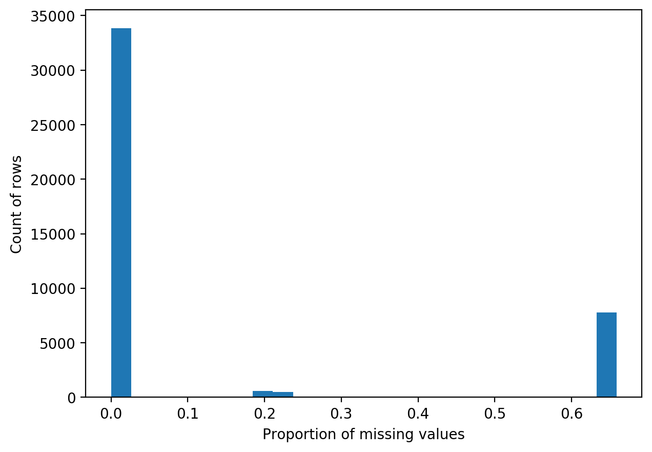
Now that all the missing values are accounted for, I plotted the count of missing values in each column in a histogram:

現在已經考慮了所有缺失值，我在直方圖中繪制了每列中缺失值的計數：

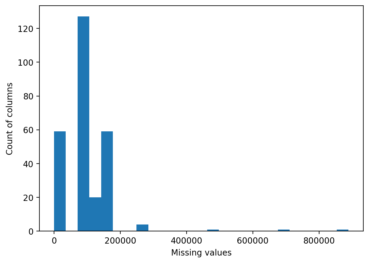
Bases on the histogram I removed cloumns with more than 200000 missing value. I also check for missing values on the row level.

根據直方圖，我刪除了缺失值超過200000的克隆。 我還檢查行級別的缺失值。

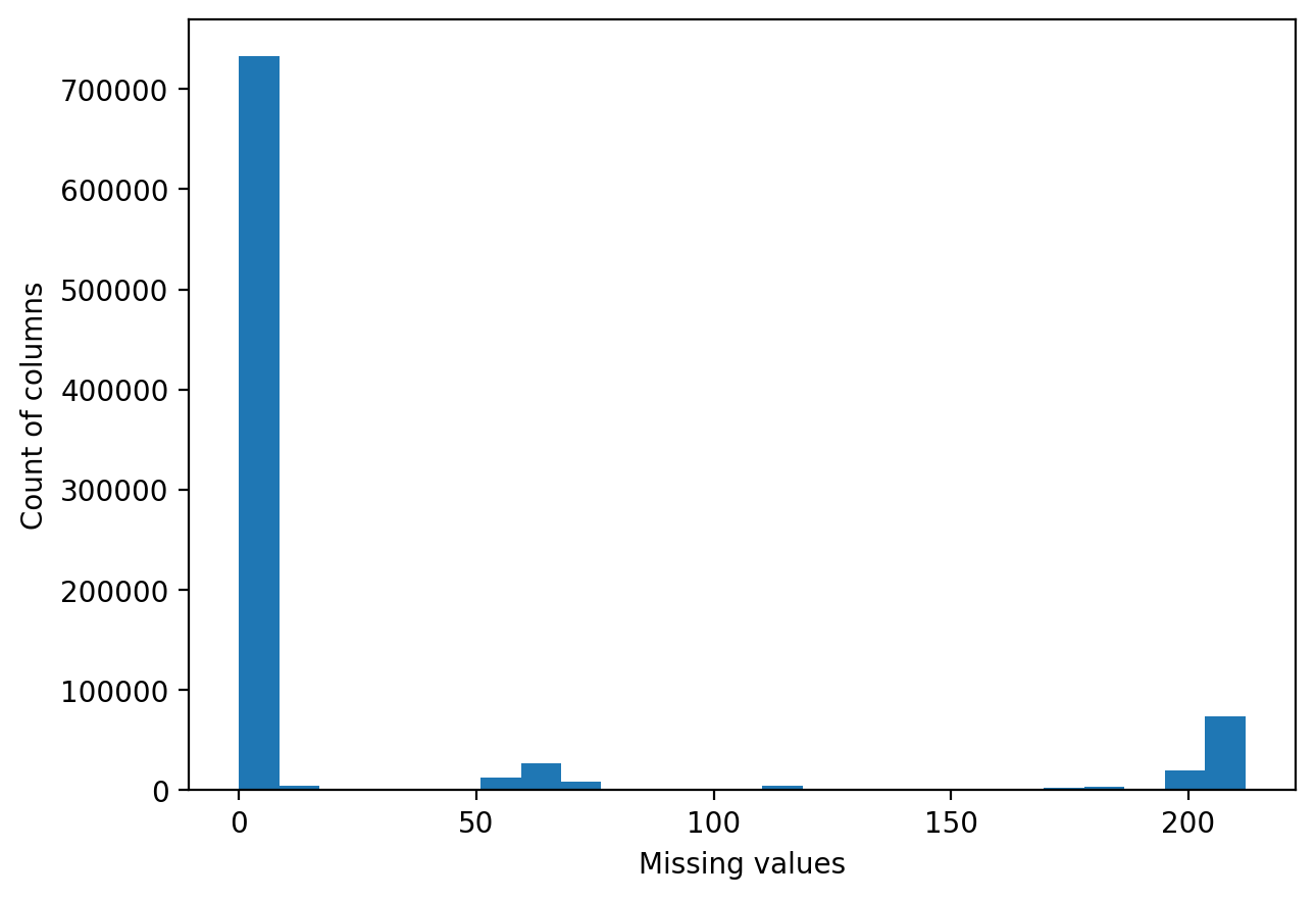
Based on this histogram I decided to remove columns that had more than 50 missing values. So all in all I removed 7 columns and 153955 rows.

基于此直方圖，我決定刪除缺失值超過50的列。 因此，我總共刪除了7列和153955行。

Check non-numeric attributes

檢查非數字屬性

If I want to use the attributes in the learning algorithms, I need to make sure that all of them are numeric. The following attributes were marked as objects.

如果要在學習算法中使用屬性，則需要確保所有屬性都是數字。 以下屬性被標記為對象。

• CAMEO_DEU_2015: detailed classification variable with more than 44 items on the scale
  CAMEO_DEU_2015：詳細的分類變量，具有超過44個項目
• CAMEO_DEUG_2015: classification variable for social status with 9 items but encoded in different dtypes (int and floats in the same column) and some rows contained XX
  CAMEO_DEUG_2015：具有9個項目的社會地位分類變量，但以不同的dtypes編碼(int和float在同一列中)，并且某些行包含XX
• OST_WEST_KZ: indication for former region (West-Germany, Ost-Germany) encoded with W and O
  OST_WEST_KZ：以W和O編碼的先前區域(西德，東德)的指示

I made the necessary transformations to CAMEO_DEUG_2015 and OST_WEST_KZ and decided to drop CAMEO_DEU_2015, because there were to many items.

我對CAMEO_DEUG_2015和OST_WEST_KZ進行了必要的轉換，并決定刪除CAMEO_DEU_2015，因為其中有很多項目。

Now that all of the attributes are numeric, I manually checked for categorical data that needed to be transformed to dummy variables. I discovered 11 categorical features:

現在，所有屬性都是數字屬性，我手動檢查了需要轉換為虛擬變量的分類數據。 我發現了11個分類功能：

• ANREDE_KZ, CJT_GESAMTTYP, GEBAEUDETYP, GEBAEUDETYP_RASTER, HEALTH_TYP, KBA05_HERSTTEMP, KBA05_MAXHERST, KBA05_MODTEMP, NATIONALITAET_KZ, SHOPPER_TYP, VERS_TYP
  ANREDE_KZ，CJT_GESAMTTYP，GEBAEUDETYP，GEBAEUDETYP_RASTER，HEALTH_TYP，KBA05_HERSTTEMP，KBA05_MAXHERST，KBA05_MODTEMP，NATIONALITAETET_KZ，SHOPPER_TYP，VERS_TYP

In the same step I also noted which attributes need to be dropped, because they would add to much complexity to the model (mainly attributes with a scale higher than 10)

在同一步驟中，我還指出了需要刪除哪些屬性，因為它們會增加模型的復雜性(主要是比例大于10的屬性)

• GFK_URLAUBERTYP, LP_FAMILIE_FEIN, LP_LEBENSPHASE_GROB, LP_FAMILIE_GROB, LP_LEBENSPHASE_FEIN
  GFK_URLAUBERTYP，LP_FAMILIE_FEIN，LP_LEBENSPHASE_GROB，LP_FAMILIE_GROB，LP_LEBENSPHASE_FEIN

Now with the main cleaning steps finished I created a function that cleaned the dataset with the customers data (Udacity_CUSTOMERS_052018.csv). For the next steps it is very important that both datasets have the same shape and columns. I had to remove one column that was created as a dummy variable from the customers dataset ‘GEBAEUDETYP_5.0’.

現在完成了主要的清理步驟，我創建了一個使用客戶數據清理數據集的函數(Udacity_CUSTOMERS_052018.csv)。 對于后續步驟，兩個數據集具有相同的形狀和列非常重要。 我必須從客戶數據集“ GEBAEUDETYP_5.0”中刪除作為虛擬變量創建的一列。

Imputation and scaling features

插補和縮放功能

To use columns with missing values I imputed the median for each column. I decided to use the median, because most of the attributes are ordinal scaled, which means that they are categorical but have a quasi linear context. In that case the median is ‘best’ way to impute

為了使用缺少值的列，我估算了每列的中位數。 我決定使用中位數，因為大多數屬性都是按序縮放的，這意味著它們是分類的，但具有準線性上下文。 在這種情況下，中位數是“最佳”估算方式

The second to last thing I did in the preprocessing step was to scale the features. I used to standardize them, which means that the new data has a mean of 0 and a std of 1.

我在預處理步驟中所做的倒數第二件事是縮放功能。 我曾經將它們標準化，這意味著新數據的平均值為0，std為1。

And finally, the last thing I did was to eliminate columns that had a correlation above 0.95.

最后，我要做的最后一件事是消除相關性高于0.95的列。

• KBA13_HERST_SONST, KBA13_KMH_250, LP_STATUS_GROB, ANREDE_KZ_2.0, KBA05_MODTEMP_5.0
  KBA13_HERST_SONST，KBA13_KMH_250，LP_STATUS_GROB，ANREDE_KZ_2.0，KBA05_MODTEMP_5.0

2.使用無監督學習算法進行客戶細分 (2. Use unsupervised learning algorithms to perform customer segmentation)

The first objective was to reduce the dimensions. After the preprocessing step I still had close to 300 features. To reduce dimensionality, we can use Principal Component Analysis. PAC uses Singular Value Decomposition of the data to project it onto a lower dimensional space. Simply put, it reduces the complexity of a high feature model.

第一個目標是減小尺寸。 在預處理步驟之后，我仍然擁有近300個功能。 為了降低維數，我們可以使用主成分分析。 PAC使用數據的奇異值分解將其投影到較低維度的空間上。 簡而言之，它降低了高功能模型的復雜性。

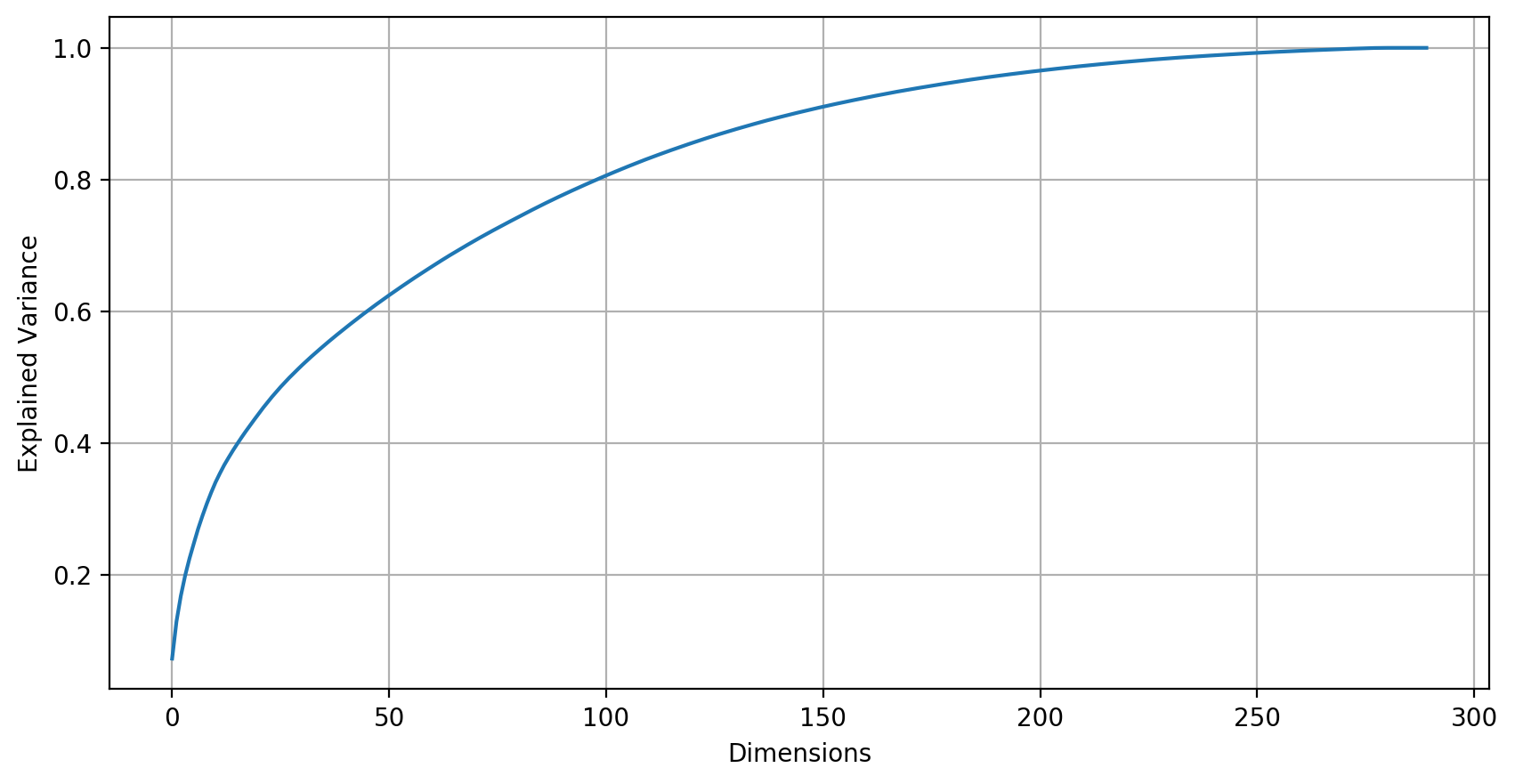
According to the book ‘Hands on Machine Learning’, it is important to choose a number of dimensions that add up to a sufficiently large portion of variance, like 95%. So, in this case I can reduce the number of dimensions by roughly 50% down to 150.

根據《機器學習的動手》一書，選擇許多維數非常重要，這些維加起來需要足夠大的方差，例如95％。 因此，在這種情況下，我可以將尺寸數量減少大約50％，減少到150。

I will briefly explain the first three competent to give an idea what they are about. I printed the top positve and negative weights for each component:

我將簡要解釋前三名主管，以給出他們的想法。 我打印了每個組件的最高位置和負重量：

Principal Component 1

主要成分1

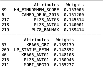
The first component is mainly related with wealth, status and number of family houses in region(PLZ8):

第一部分主要與該地區的家庭財產，地位和數量有關(PLZ8)：

• HH_EINKOMMEN_SCORE: estimated household income
  HH_EINKOMMEN_SCORE：估計的家庭收入
• CAMEO_DEUG_2015: social status of the individual (upper class -> urban working class)
  CAMEO_DEUG_2015：個人的社會地位(上層階級->城市工人階級)
• PLZ8_ANTG1/3/4: number of family houses in the neighborhood
  PLZ8_ANTG1 / 3/4：附近的家庭住宅數量
• MOBI_REGIO: moving patterns (high mobility -> very low mobility)
  MOBI_REGIO：移動模式(高移動性->低移動性)
• LP_Status_FEIN: social status (typical low-income earners -> top earners)
  LP_Status_FEIN：社會地位(典型的低收入者->最高收入者)

Principal Component 2

主要組成部分2

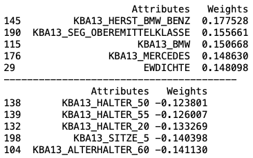
The second component is related to cars:

第二部分與汽車有關：

• KBA13_HERST_BMW_BENZ: share of BMW & Mercedes Benz within the PLZ8
  KBA13_HERST_BMW_BENZ：PLZ8中寶馬和奔馳的份額
• KBA13_SEG_OBERMITTELKLASSE: share of upper middle-class cars and upper-class cars (BMW5er, BMW7er etc.)
  KBA13_SEG_OBERMITTELKLASSE：上等中產車和上等車(BMW5er，BMW7er等)的份額
• KBA13_HALTER_50/55/20: age of car owner
  KBA13_HALTER_50 / 55/20：車主的年齡

Principal Component 3

主要組成部分3

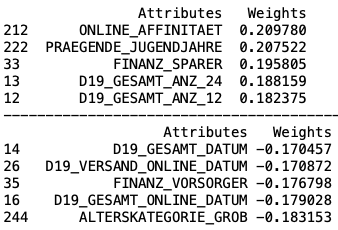
The third component is related to age, financial decisions and transactions:

第三部分與年齡，財務決策和交易有關：

• PRAEGENDE_JUGENDJAHRE: dominating movement in the person’s youth (avantgarde or mainstream)
  PRAEGENDE_JUGENDJAHRE：在青年時代(前衛或主流)主導運動
• FINANZ _SPARER: financial typology: money saver (very high -> very low)
  FINANZ _SPARER：財務類型：省錢(非常高->非常低)
• D19_GESAMT_ANZ_24: transaction activity TOTAL POOL in the last 24 months (no transaction -> very high activity)
  D19_GESAMT_ANZ_24：過去24個月的交易活動總計TOTAL POOL(無交易->交易量很高)
• FINANZ_VORSORGER: financial typology be prepared (very high -> very low)
  FINANZ_VORSORGER：準備財務類型(非常高->非常低)
• ALTERSKATEGORIE_GROB: age classification through prename analysis
  ALTERSKATEGORIE_GROB：通過姓氏分析進行年齡分類

聚類 (Clustering)

Now that we reduced the number of dimensions in both datasets and get a brief understanding of the first components, it is time to cluster them to see if there are any differences between the clusters from the general population and the ones from the customers population. To achievethis, I will use KMeans.

現在，我們減少了兩個數據集中的維數，并簡要了解了第一個組件，是時候對它們進行聚類了，以查看來自一般總體的聚類和來自客戶總體的聚類之間是否存在差異。 為此，我將使用KMeans。

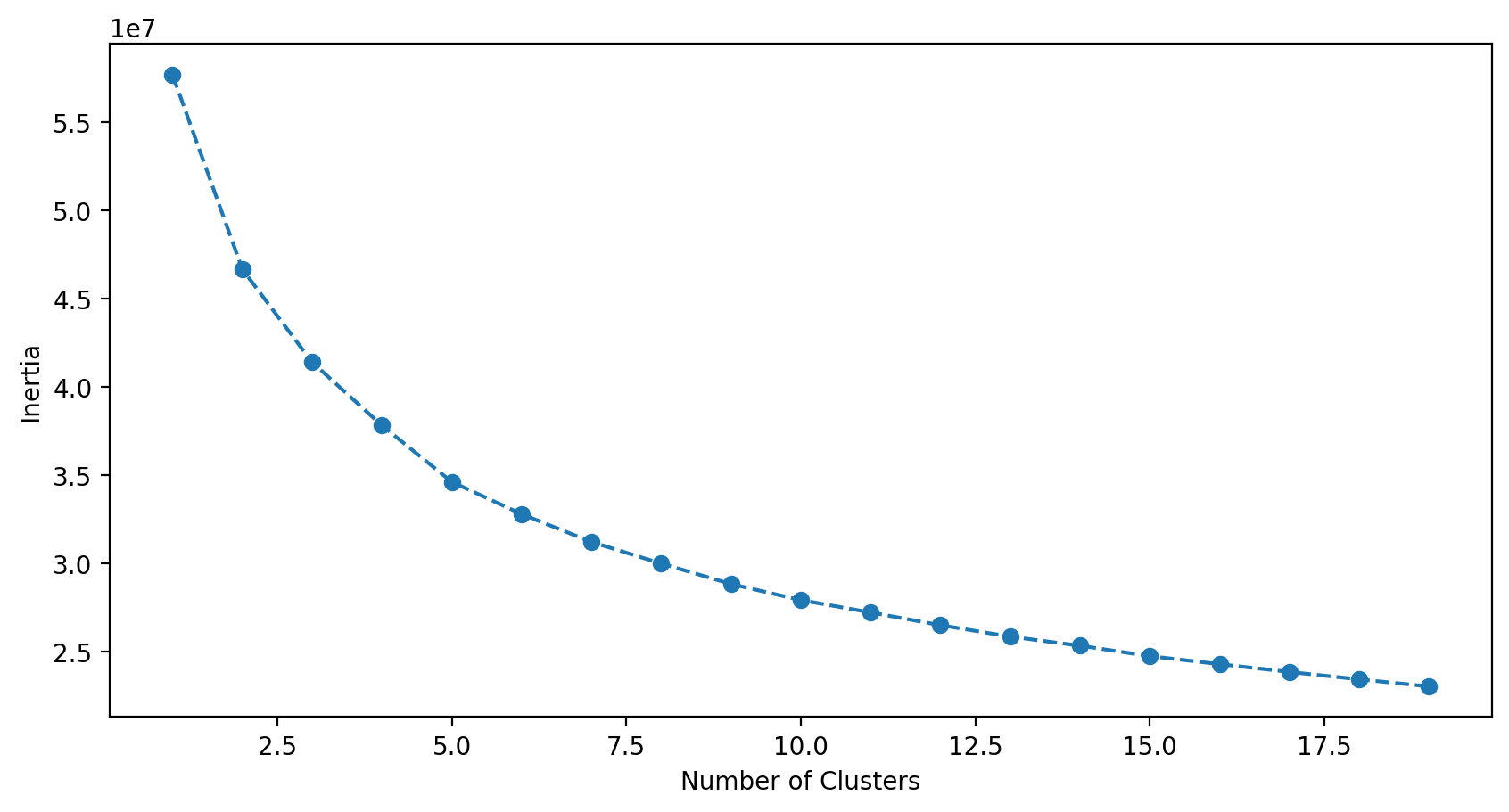
We can use the ‘Elbow’-method to get ‘right’ number of clusters. An ‘Elbow’ is defined as the point in the above chart where the decrease in Inertia almost flattens. In my case there isn’t a clear ‘Elbow’ point. 10 seems to be a good choice to have enough clusters to compare against but not too much to add unnecessary complexity.

我們可以使用“肘”方法來獲得“正確的”簇數。 上圖中的“肘”定義為慣性下降幾乎趨于平穩的點。 就我而言，沒有明確的“肘”點。 10有足夠的集群進行比較似乎是一個不錯的選擇，但又不要過多，以免增加不必要的復雜性。

Comparing AZDIAS cluster with CUSTOMERS cluster

比較AZDIAS集群和CUSTOMERS集群

It is clear to see that almost every cluster differentiate between the customers and the general population. When looking at the bars we can easily see which cluster is overrepresented by the customers, which means that customers can be described by the features for that cluster. Customers can be described with the features from cluster 0, 7and 6.

顯而易見，幾乎每個集群都在客戶和普通人群之間有所區別。 當查看條形圖時，我們可以輕松地看到客戶代表了哪個集群，這意味著可以通過該集群的功能來描述客戶。 可以使用群集0、7和6中的功能描述客戶。

We can also describe individuals that won’t become our customers, when we are looking at the clusters where the population is overrepresented, like cluster 8, 3 and 9.

當我們查看人口過多的集群時，例如集群8、3和9，我們還可以描述不會成為客戶的個人。

The main customers of the company

公司主要客戶

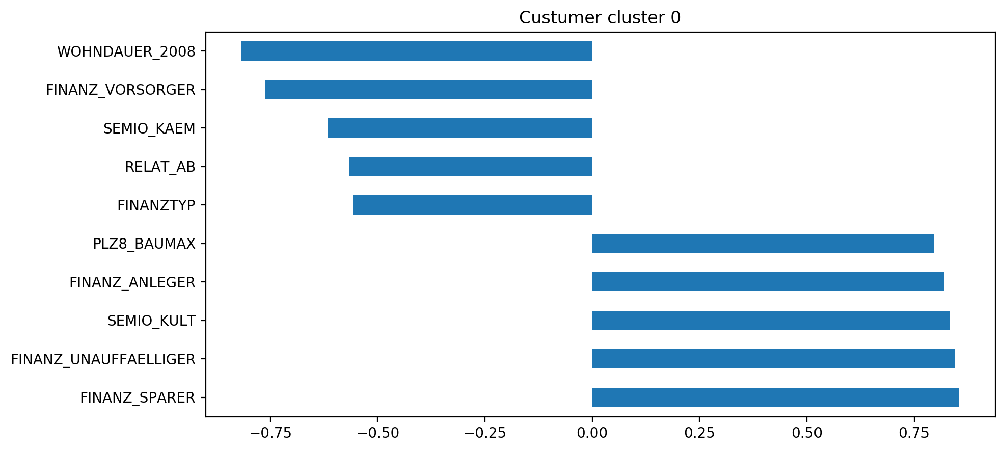
An individual part of that clusters 0:

該部分的單個部分聚集為0：

• lives in an area with mostly family homes and low unemployment
  生活在大部分家庭住宅和低失業率的地區
• has a higher affinity for a fightfull attitude and is financial prepared.
  對斗志滿滿的態度有較高的親和力，并且有充分的財務準備。
• but has low financial interest, is not an investor and not good with saving money
  但經濟利益低，不是投資者，也不擅長存錢
• not really culturally minded
  沒有真正的文化意識

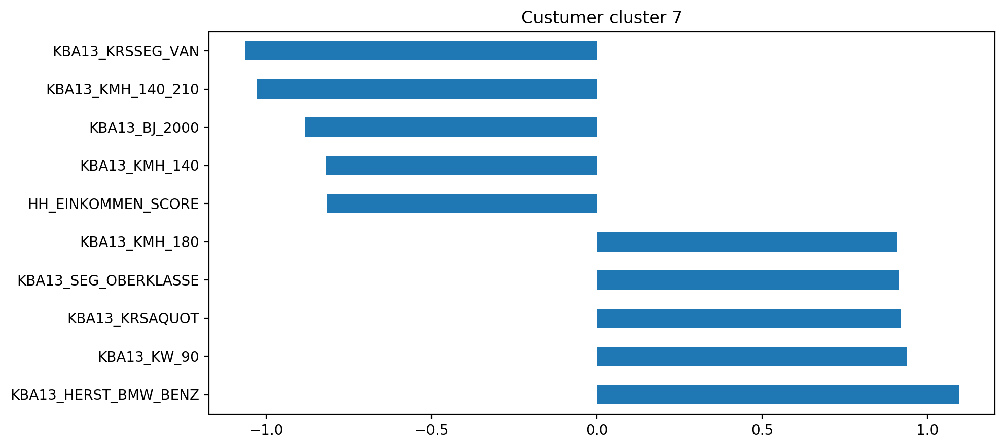
An individual part of clusters 7 is mainly described by its car choice:

集群7的單個部分主要通過其汽車選擇來描述：

• has a high income and a high share of upper class cars (BMW 7er etc)
  收入高，高檔轎車比例高(寶馬7er等)
• high share of cars per household
  每個家庭的汽車占有率很高
• very few cars with a max speed between 110 and 210 and were built between 2000 and 2003, so mostly new cars
  在2000年至2003年之間生產的極少數汽車的最高速度在110至210之間
• has in his area a lot less vans, compared to country average
  與全國平均水平相比，他所在地區的貨車少很多

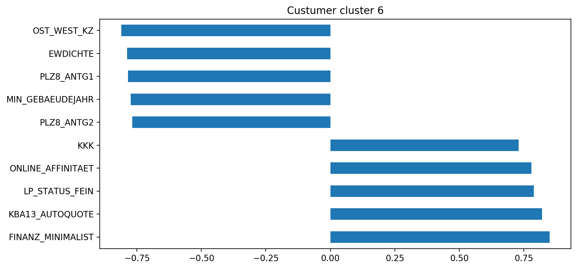
An individual part of this cluster 6:

該集群的一部分6：

• lives in a low density area in an old building, with only a few family houses around
  住在一棟舊樓的低密度區域，周圍只有幾戶人家
• has low purchasing power but still a higher car share per household
  購買力低，但每個家庭的汽車份額仍然較高
• is more minimalistic / independent
  更簡約/獨立
• low financial interest
  財務利益低
• high online affinity
  網上親和力高

Now lets look at clusters where customers are underrepressented

現在，讓我們看看客戶壓力不足的集群

An individual part of this cluster 8:

該集群的一部分8：

• has high purchasing power, but has a lower income
  具有較高的購買力，但收入較低
• is part of the lower middle-class / working-class
  是下層中產階級/工人階級的一部分
• has a low number of family homes in the area
  該地區的家庭住宅數量少
• low online affinity and share of cars per household
  在線親和力低，每戶擁有汽車的比例低
• low car share per household
  每個家庭的汽車占有率低

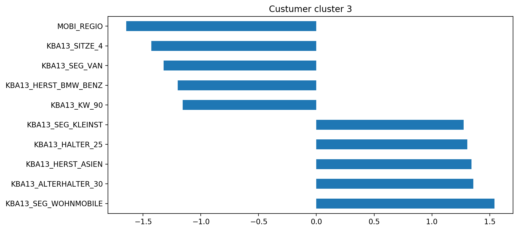
An individual part of this cluster 3:

該集群的一部分：

• has high mobility, but a low number of cars with less than 5 seats
  機動性高，但座位數少于5的汽車數量少
• dives mostly small cars (high number of very small cars (Ford Fiesta, Ford Ka) and low number of BMW and Mercedes)
  大多潛水小型車(大量的小型車(福特嘉年華，福特嘉年華)和少量的寶馬和梅賽德斯)
• is mostly between 21 and 25 and drives cars from Asian manufactures
  通常在21至25歲之間，并駕駛來自亞洲制造商的汽車
• high share hare of car owners below 31 within the PLZ8
  PLZ8以內31歲以下車主的高份額野兔
• and interestingly high amount of campers
  有趣的是，大量的露營者

For cluster 9 it is almost the same.

對于群集9，幾乎是相同的。

3.使用監督學習算法來預測個人是否會成為客戶 (3. Use supervised learning algorithms to predict if am individual will become a customer)

Now that I have found which parts of the population are more likely to be customers of the mail-order company, it’s time to build the prediction model.

現在，我已經發現人口中的哪些部分更可能成為郵購公司的客戶，是時候建立預測模型了。

I used the provided dataset Udacity_MAILOUT_052018_TRAIN.csv to train various models, select the best one and did some hyper-parameter tuning to increase the effectiveness of my model. But first I had to clean the data.

我使用提供的數據集Udacity_MAILOUT_052018_TRAIN.csv來訓練各種模型，選擇最佳模型，并進行一些超參數調整，以提高模型的有效性。 但是首先我必須清理數據。

The cleaning was relatively simple because I can use the cleaning function created in the first part of the project. After that I check missing values:

清理相對簡單，因為我可以使用在項目的第一部分中創建的清理功能。 之后，我檢查缺少的值：

Based on the histograms I decided to only drop rows with more than 30% missing values.

根據直方圖，我決定只刪除缺失值超過30％的行。

To use the data for the learning algorithm I imputed the median, standardized the data and dropped highly correlated features (>0.95). In each step where I dropped columns, I made sure that I dropped the same columns in the test set (Udacity_MAILOUT_052018_TEST.csv) to make predictions on this unseen dataset.

為了將數據用于學習算法，我估算了中位數，對數據進行了標準化，并刪除了高度相關的特征(> 0.95)。 在放置列的每個步驟中，確保將相同的列都放置在測試集中(Udacity_MAILOUT_052018_TEST.csv)，以便對該看不見的數據集進行預測。

Finally, the fun part begins: creating the model and male predictions.

最后，有趣的部分開始：創建模型和男性預測。

First, I check the distribution of the relevant variable ‘RESPONSE’. As it turns out ‘RESPONSE’ is highly imbalanced: 0: 34565 and 1: 435.

首先，我檢查相關變量“ RESPONSE”的分布。 事實證明，“響應”高度不平衡：0：34565和1：435。

If the variable of interest is imbalanced it is important to make sure of the following things:

如果感興趣的變量不平衡，請確保以下幾點很重要：

• use stratification for the tranig and validation set: Stratification is a technique to distribute the samples evenly based on sample classes so that training set and validation set have similar ratio of classes.
  對成績單和驗證集使用分層：分層是一種根據樣本類別均勻分配樣本的技術，以便訓練集和驗證集具有相似的類別比率。

• choose the right evaluation metric: Simply choose accuracy won’t give you ‘accurate’ evaluations. The best one in this case would be the roc-auc socre This article explains it.

  選擇正確的評估指標：僅選擇準確性不會給您“準確”的評估。 在這種情況下最好的是roc-auc socre 本文對此進行了解釋。

• use a gradient boosting algorithm: I will run multiple classification algorithms and choose the best one
  使用梯度提升算法：我將運行多種分類算法并選擇最佳的算法

There are also some advanced techniques to deal with it that I wpn’t implement. You can read about it here.

還有一些我不會實現的高級技術。 你可以在這里閱讀。

Classification algorithms

分類算法

I tested the following classifications algorithms in a cross validation method:

我以交叉驗證方法測試了以下分類算法：

• LogisticRegression
  Logistic回歸
• DecisionTreeClassifier
  DecisionTreeClassifier
• RandomForestClassifier
  隨機森林分類器
• AdaBoostClassifier
  AdaBoostClassifier
• GradientBoostingClassifier
  梯度提升分類器

I used sklearns StratifiedKFold method to make sure I used stratification when doing the evaluation of the classifiers.

我使用sklearns StratifiedKFold方法來確保在評估分類器時使用分層。

I created a pipeline where each model in the classifier dictionary gets evaluated on the ‘roc_auc’ scoring technique.

我創建了一個管道，分類器字典中的每個模型都可以通過“ roc_auc”評分技術進行評估。

Results

結果

• LogisticRegression: 0.5388771114225904
  Logistic回歸：0.5388771114225904
• DecisionTreeClassifier: 0.5065447241661969
  DecisionTreeClassifier：0.5065447241661969
• RandomForestClassifier: 0.5025457616916987
  隨機森林分類器：0.5025457616916987
• AdaBoostClassifier: 0.5262902976401282
  AdaBoostClassifier：0.5262902976401282
• GradientBoostingClassifier: 0.5461740415775044
  梯度提升分類器：0.5461740415775044

As expected, the classifier using gradiant boosting git the best result. In the next step I used GridSearch to find the best Hyperparameters for the GradientBoostingClassifier

不出所料，使用gradient boosting git的分類器效果最佳。 在下一步中，我使用GridSearch來找到GradientBoostingClassifier的最佳超參數

With all other options on normal:

在所有其他選項均正常的情況下：

• learning_rate: 0.1
  學習率：0.1
• max_death: 5
  max_death：5
• n_estimators: 200
  n_estimators：200

I increased the score from 0.546 to 0.594.

我將分數從0.546提高到0.594。

4.對看不見的數據集進行預測，然后將結果上傳到Kaggle (4. Make prediction on an unseen dataset and upload result to Kaggle)

Now that I tuned and trained the best model I can finally make predictions on the unseen dataset (Udacity_MAILOUT_052018_TEST.csv).

現在，我已經調整和訓練了最佳模型，我終于可以對看不見的數據集(Udacity_MAILOUT_052018_TEST.csv)進行預測。

For the final part I just had to impute the missing values and standardize the new dataset, made sure that the columns were the same and run the trained model on the new data.

對于最后一部分，我只需要估算缺少的值并標準化新數據集，請確保列相同，然后對新數據運行經過訓練的模型。

I transformed the output to the requirements of the Kaggle competition and uploaded my submission file.

我將輸出轉換為Kaggle競賽的要求，并上傳了提交文件。

I got a score of 0.536 in the Kaggle Competitio.

我在Kaggle競賽中獲得0.536分。

結論 (Conclusions)

To recap, the first goal of this project was to perform an unsupervised learning algorithm to uncover differences between customers and the general population. The second goal was to perform a supervised learning algorithm to predict if an individual became a customer and the last goal was to use this trained model to predict on unseen data and upload the results to Kaggle.

回顧一下，該項目的第一個目標是執行一種無監督的學習算法，以發現客戶與一般人群之間的差異。 第二個目標是執行監督學習算法，以預測個人是否成為客戶，最后一個目標是使用經過訓練的模型來預測看不見的數據，并將結果上傳到Kaggle。

The first part (unsupervised learning) was very challenging for me. It was the first time that I worked with a huge datafile (> 1GB). So, at first it was quite frustrating working on the provided workspace, since some operations took a while. I decided to download the data to work on it on my local machine.

第一部分(無監督學習)對我來說非常具有挑戰性。 這是我第一次使用巨大的數據文件(> 1GB)。 因此，起初，在提供的工作空間上進行工作非常令人沮喪，因為某些操作花費了一段時間。 我決定下載數據以在本地計算機上進行處理。

Besides the huge dataset, the data cleaning was also very challenging, and I used quite frequently methods that I didn’t used before, so it was on the other side quite rewarding to implement a new method and get the expected result.

除了龐大的數據集之外，數據清理也非常具有挑戰性，我經常使用以前從未使用過的方法，因此，另一方面，實施一種新方法并獲得預期結果也頗有收獲。

Again, it became clear that the most work a data scientist has is the cleaning step.

同樣，很明顯，數據科學家要做的最大工作就是清理步驟。

局限性 (Limitations)

My final score is compared to others on Kaggle relatively low. I looked at a few other notebooks on github to get an idea why. It seems that my approach, to only keep the columns that are in the dataset and in the excel file is quite unique. To recap, I dropped 94 columns that weren’t in both files, with the idea that I can only use attributes for which I have the description. After the analysis I inspected the excel file and noticed that some Attributes are just spelled differently between the excel file and the dataset. So, all in all I probably dropped some columns that meight would increase my score.

我的最終成績與Kaggle上的其他人相比較低。 我查看了github上的其他筆記本以了解原因。 看來，僅保留數據集中和excel文件中的列的方法非常獨特。 回顧一下，我刪除了兩個文件中都沒有的94列，以為我只能使用具有描述的屬性。 分析之后，我檢查了excel文件，發現excel文件和數據集之間的某些屬性拼寫有所不同。 因此，總的來說，我可能會丟掉一些可能會增加得分的列。

Another thing that I noticed is that I dropped rows in the supervised learning part. Which is debatable because the variable of interest is to highly imbalanced and one can argue that it would be better to keep rows with missing values, so that there is a higher chance for the imbalanced value to appear.

我注意到的另一件事是，我在有監督的學習部分中刪除了行。 這是值得商because的，因為關注變量的高度不平衡，并且有人可能會說最好保留值缺失的行，這樣就更有可能出現不平衡的值。

All in all, here are some things that could be checked to enhance the final score:

總而言之，以下是可以提高最終得分的一些事情：

• get a better understanding of the attributes and check if you can use more attributes without dropping them (keep attributes with more than 10 items)
  更好地了解屬性，并檢查是否可以使用更多屬性而不刪除它們(保留包含10個以上項目的屬性)
• don’t drop attributes because they aren’t in the Excel file
  不要刪除屬性，因為它們不在Excel文件中
• use more advanced methods to impute missing values (imputations based on distributions ore even use a learning algorithm to predict the missing value)
  使用更高級的方法來估算缺失值(基于分布礦的算力甚至使用學習算法來預測缺失值)
• use more advanced techniques to deal with imbalanced data (Resampling to get more balanced data, weighted classes / cost sensitive learning).
  使用更先進的技術來處理不平衡的數據(重新采樣以獲得更平衡的數據，加權類/對成本敏感的學習)。

If you are interested in the code, you can take a look at this Github repo.

如果您對代碼感興趣，可以查看此 Github存儲庫。