這次實踐的前半部分是，用水庫水位的變化，來預測大壩的出水量。
給數據集擬合一條直線，可能得到一個邏輯回歸擬合，但它并不能很好地擬合數據，這是高偏差（high bias）的情況，也稱為“欠擬合”（underfitting）
相反，如果我們擬合一個非常復雜的分類器，比如深度神經網絡或含有隱藏單元的神經網絡，可能非常適用于這個數據，但是這看起來也不是一種很好的擬合方式分類器----方差較高（high variance）
數據過擬合（over fitting）

• 高偏差和高方差是兩種不同的情況，通常會用訓練驗證集來診斷算法是否存在偏差或方差問題。
• 在機器學習初級階段，會有很多關于偏差方差的討論，能嘗試的方法很多。在當前深度學習和大數據時代，只需持續訓練更大的網絡，就能不影響方差減少偏差；準備更多的數據，就能不影響偏差減少方差。

Regularized Linear Regression

Visualizing the dataset

data = loadmat('ex5data1.mat')
# Training set
X, y = data['X'], data['y']
# Cross validation set
Xval, yval = data['Xval'], data['yval']
# Test set
Xtest, ytest = data['Xtest'], data['ytest']X = np.insert(X, 0, 1, axis=1)
Xval = np.insert(Xval, 0, 1, axis=1)
Xtest = np.insert(Xtest, 0, 1, axis=1)def plot_data():plt.figure(figsize=(6, 4))plt.scatter(X[:, 1:], y, c='r', marker='x')plt.xlabel('change in water level(x)')plt.ylabel('Water flowing out of the dam (y)')plt.grid(True)plot_data()
plt.show()

Regularized linear regression cost function

def regularized_cost(theta, X, y, l):cost = ((X.dot(theta) - y.flatten()) **2).sum()/(2*len(X))regularized_theta = l * (theta[1:].dot(theta[1:]))/(2 * len(X))return cost + regularized_thetatheta = np.ones(X.shape[1])
print(regularized_cost(theta, X, y, 1))

Regularized linear regression gradient

def regularized_gradient(theta, X, y, l):grad = (X.dot(theta) - y.flatten()).dot(X)regularized_theta = l * thetareturn (grad + regularized_theta) / len(X)print(regularized_gradient(theta, X, y, 1))

def train_linear_regularized(X, y, l):theta = np.zeros(X.shape[1])res = opt.minimize(fun=regularized_cost,x0=theta,args=(X, y, l),method='TNC',jac=regularized_gradient)return res.x

Fitting linear regression

擬合線性回歸，畫出擬合線

final_theta = train_linear_regularized(X, y, 0)
plot_data()
plt.plot(X[:, 1], X.dot(final_theta))
plt.show()

Bias-variance

Learning curves

畫出學習曲線

def plot_learning_curve(X, y, Xval, yval, l):training_cost, cross_cost = [], []for i in range(1, len(X)):res = train_linear_regularized(X[:i], y[:i], l)training_cost_item = regularized_cost(res, X[:i], y[:i], 0)cross_cost_item = regularized_cost(res, Xval, yval, 0)training_cost.append(training_cost_item)cross_cost.append(cross_cost_item)plt.figure(figsize=(6, 4))plt.plot([i for i in range(1, len(X))], training_cost, label='training cost')plt.plot([i for i in range(1, len(X))], cross_cost, label='cross cost')plt.legend()plt.xlabel('Number of training examples')plt.ylabel('Error')plt.title('Learning curve for linear regression')plt.grid(True)plot_learning_curve(X, y, Xval, yval, 0)
plt.show()

Polynomial regression

Learning Polynomial Regression

使用多項式回歸，規定假設函數如下：

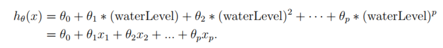
def genPolyFeatures(X, power):Xpoly = X.copy()for i in range(2, power + 1):Xpoly = np.insert(Xpoly, Xpoly.shape[1], np.power(Xpoly[:,1], i), axis=1)return Xpoly#獲取訓練集的均值和誤差
def get_means_std(X):means = np.mean(X, axis=0)stds = np.std(X, axis=0, ddof=1) # ddof=1  樣本標準差return means, stds# 標準化
def featureNormalize(myX, means, stds):X_norm = myX.copy()X_norm[:,1:] = X_norm[:,1:] - means[1:]X_norm[:,1:] = X_norm[:,1:] / stds[1:]return X_normpower = 6  # 擴展到x的6次方train_means, train_stds = get_means_std(genPolyFeatures(X,power))
X_norm = featureNormalize(genPolyFeatures(X,power), train_means, train_stds)
Xval_norm = featureNormalize(genPolyFeatures(Xval,power), train_means, train_stds)
Xtest_norm = featureNormalize(genPolyFeatures(Xtest,power), train_means, train_stds)def plot_fit(means, stds, l):"""擬合曲線"""theta = train_linear_regularized(X_norm, y, l)x = np.linspace(-75, 55, 50)xmat = x.reshape(-1, 1)xmat = np.insert(xmat, 0, 1, axis=1)Xmat = genPolyFeatures(xmat, power)Xmat_norm = featureNormalize(Xmat, means, stds)plot_data()plt.plot(x, Xmat_norm @ theta, 'b--')plot_fit(train_means, train_stds, 0)
plot_learning_curve(X_norm, y, Xval_norm, yval, 0)

Adjusting the regularization parameter

plot_fit(train_means, train_stds, 1)
plot_learning_curve(X_norm, y, Xval_norm, yval, 1)
plt.show()

Selecting λ using a cross validation set

嘗試用不同的lambda調試，進行交叉驗證

lambdas = [0., 0.001, 0.003, 0.01, 0.03, 0.1, 0.3, 1., 3., 10.]
errors_train, errors_val = [], []
for l in lambdas:theta = train_linear_regularized(X_norm, y, l)errors_train.append(regularized_cost(theta, X_norm, y, 0))errors_val.append(regularized_cost(theta, Xval_norm, yval, 0))plt.figure(figsize=(8, 5))
plt.plot(lambdas, errors_train, label='Train')
plt.plot(lambdas, errors_val, label='Cross Validation')
plt.legend()
plt.xlabel('lambda')
plt.ylabel('Error')
plt.grid(True)