上一篇，結合代碼，我們詳細的介紹了YOLOV8目標跟蹤的Pipeline。大家應該對跟蹤的流程有了大致的了解，下面我們將對跟蹤中出現的卡爾曼濾波進行解讀。

1.卡爾曼濾波器介紹

卡爾曼濾波（kalman Filtering）是一種利用線性系統狀態方程，通過系統輸入觀測數據，對系統狀態進行最優估計的算法。由于觀測數據中包括系統中的噪聲和干擾的影響，所以最優估計也可看作是濾波過程。

卡爾曼濾波在測量方差已知的情況夏能夠從一系列存在測量噪聲的數據中，估計動態系統的狀態。在目標跟蹤中，將檢測框的坐標看作觀測數據，通過狀態轉移矩陣與狀態協方差矩陣來更新下一幀的最優估計。

2.卡爾曼濾波器的基本概念

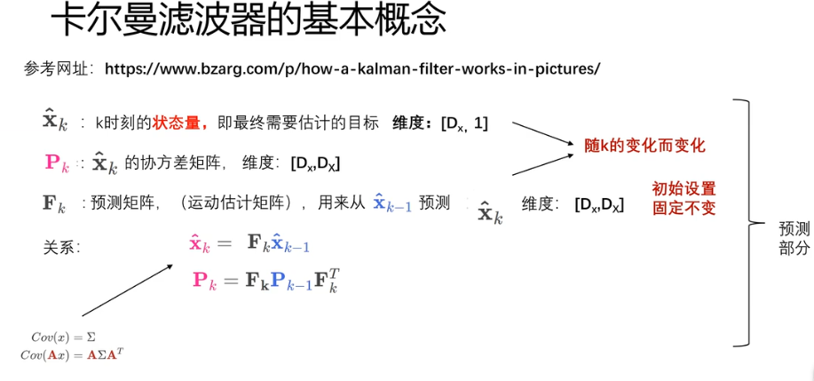
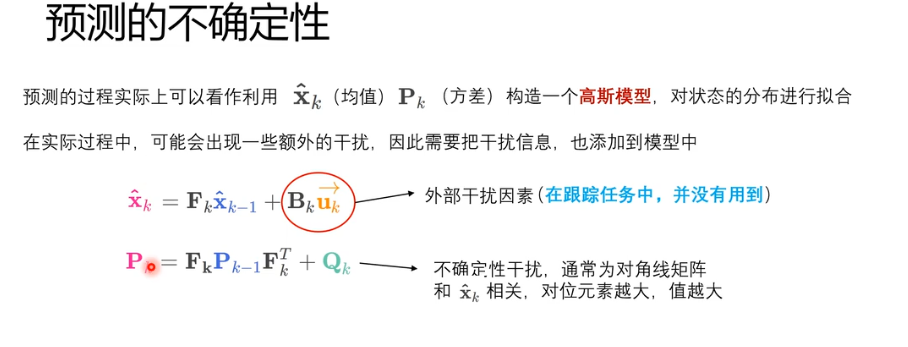
首先，我們需要了解卡爾曼濾波器的一些基本概念。$\widehat{X_k}$表示k時可的狀態量，$F_k$表示$\widehat{X_k}$的狀態轉移矩陣（運動估計矩陣）。我們可以利用$\widehat{X_{k?1}}$通過$F_k$獲得k時刻的估計$\widehat{X_k}$。$P_k$作為狀態協方差矩陣，也需要根據$F_k$更新。

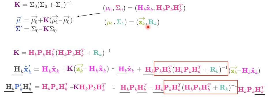
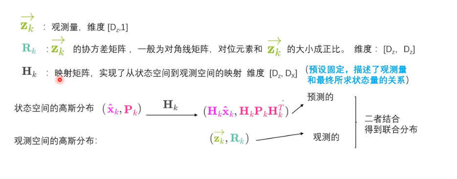觀測量與狀態量可能存在兩個不同的空間，因此需要$H_k$實現狀態空間到觀測空間的映射。由于傳感器檢測的觀測量存在誤差，我們可以把觀測空間理解為高斯分布，而狀態量本就是一種估計，相較于觀測量，狀態量可以理解為具有較大方差的高斯分布，其均值為狀態量。
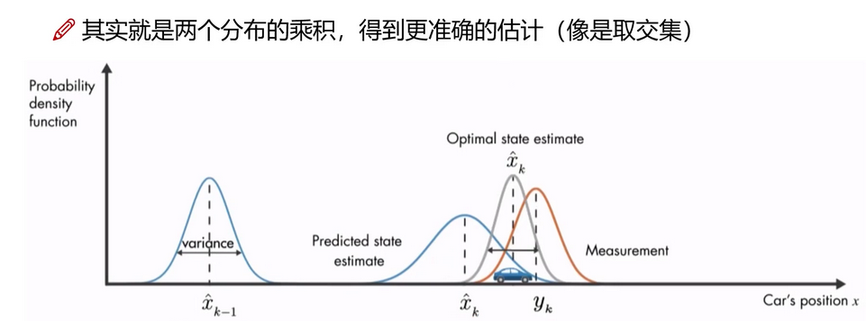如上圖所示，狀態量$\widehat{X_{k?1}}$是位于左側的高斯分布，通過狀態轉移矩陣獲得k時刻狀態量$\widehat{X_k}$，由于過程中存在各種誤差，方差較大。紅色部分是k時刻的觀測量$y_k$。由于無法預知$\widehat{X_k}$和$y_k$兩者哪邊更為準確，我們將兩者結合，得到的聯合分布看作卡爾曼濾波最后更新的狀態量。
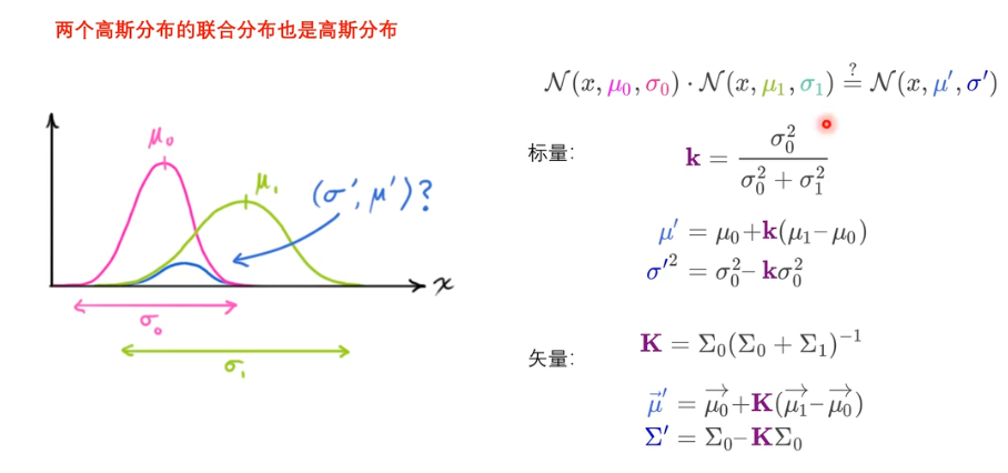
已知兩個高斯分布，其聯合分布也為高斯分布，聯合高斯分布的均值為${\hat{\mu }}^{\prime }$,${\hat{\Sigma }}^{\prime }$。

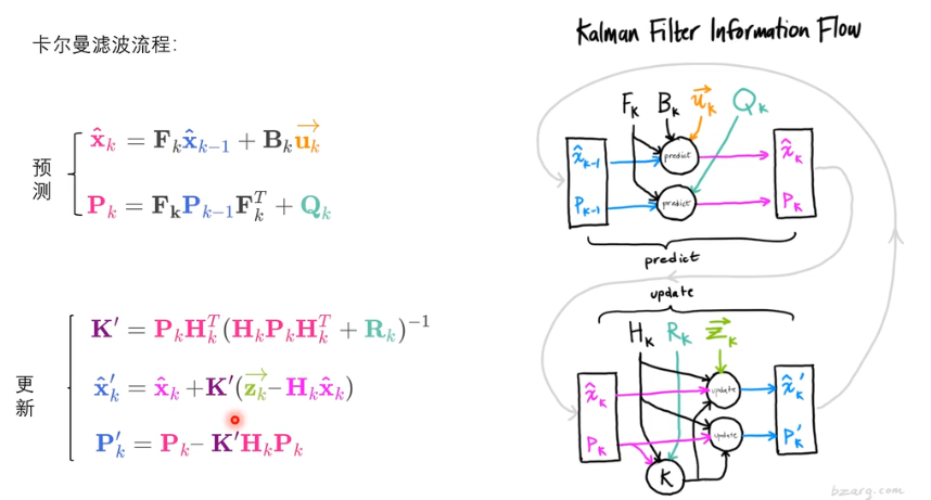
根據上圖中簡單的矩陣計算，我們得到卡爾曼濾波預測與更新5個重要公式。
預測：$P_{k?1}$,$\widehat{X_{k?1}}$根據狀態轉移矩陣獲得k時刻$\widehat{P_k}$與$\widehat{X_k}$
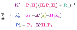
更新：將狀態量映射至觀測量空間，聯合觀測量更新狀態量${\widehat{X_k}}^{\prime }$，狀態協方差矩陣${P_k}^{\prime }$，本質是將觀測量與狀態量的高斯分布結合，形成的聯合分布看作最終狀態量的分布，其中$K^{\prime }$稱為卡爾曼增益。

3.卡爾曼濾波在目標跟蹤的應用

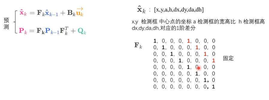首先，狀態量為[x,y,a,h,dx,dy,da,dh],我們需要預測坐標框下一幀的位置，所以狀態轉移矩陣很簡單，表示為圖中所示固定矩陣$F_k$。物理意義:下一時刻的位置=該時刻的位置+該時刻的速度×$\Delta$t，這里$\Delta$t設為1。系統輸入$u_k$設為0。

為什么選用xyah作為狀態量，而不是xyxy？主要考慮xyah作為4個獨立變量，他們的協方差=0，因此協方差矩陣可以表示為對角矩陣。而xyxy形式，左上角坐標與右小角坐標有相關性，協方差矩陣不可表示為對角矩陣。

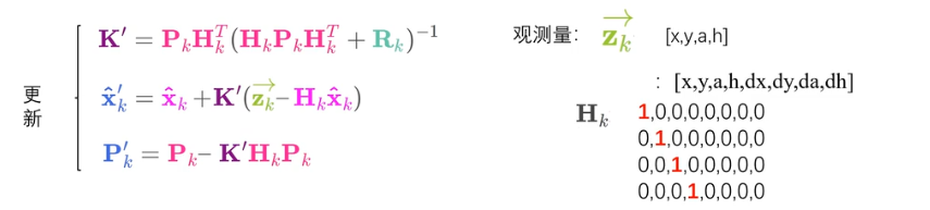
觀測量為[x,y,a,h]，因此映射矩陣$H_k$為圖中所示固定矩陣。我們對KF進行初始化，self._motion_mat表示$F_k$狀態轉移矩陣，self._update_mat表示$H_k$映射矩陣， self._std_weight_position表示位置方差的權重，self._std_weight_velocity 表示速度方差的權重，賦值均為經驗值。

def __init__(self):"""Initialize Kalman filter model matrices with motion and observation uncertainties."""ndim, dt = 4, 1.# Create Kalman filter model matrices.self._motion_mat = np.eye(2 * ndim, 2 * ndim)for i in range(ndim):self._motion_mat[i, ndim + i] = dtself._update_mat = np.eye(ndim, 2 * ndim)# Motion and observation uncertainty are chosen relative to the current# state estimate. These weights control the amount of uncertainty in# the model. This is a bit hacky.self._std_weight_position = 1. / 20self._std_weight_velocity = 1. / 160

將該幀未關聯的檢測框坐標作為新軌跡的狀態量，同時將mean_vel初始化為0。 $\widehat{X_k}$=mean = np.r_[mean_pos, mean_vel]。$P_k$初始化，其中x,y,h,$x^{\prime },y^{\prime },h^{\prime }$的方差均與h為正比，a，$a^{\prime }$為寬高比，方差為常值1e-2,1e-5。因為xy為檢測框中心點，它存在于圖中任意點，作為方差沒有意義，因此方差正比于h。

def initiate(self, measurement):"""Create track from unassociated measurement.Parameters----------measurement : ndarrayBounding box coordinates (x, y, a, h) with center position (x, y),aspect ratio a, and height h.Returns-------(ndarray, ndarray)Returns the mean vector (8 dimensional) and covariance matrix (8x8dimensional) of the new track. Unobserved velocities are initializedto 0 mean."""mean_pos = measurementmean_vel = np.zeros_like(mean_pos)mean = np.r_[mean_pos, mean_vel]std = [2 * self._std_weight_position * measurement[3], 2 * self._std_weight_position * measurement[3], 1e-2,2 * self._std_weight_position * measurement[3], 10 * self._std_weight_velocity * measurement[3],10 * self._std_weight_velocity * measurement[3], 1e-5, 10 * self._std_weight_velocity * measurement[3]]covariance = np.diag(np.square(std))return mean, covariance

在進行軌跡關聯前，需要預測軌跡在該幀的狀態量。上面我們已經討論了卡爾曼濾波預測的公式，翻譯成代碼就如下所示，其中motion_cov表示不確定性干擾，通常為對角矩陣狀態量相關，對位元素越大，其值越大。

def predict(self, mean, covariance):"""Run Kalman filter prediction step.Parameters----------mean : ndarrayThe 8 dimensional mean vector of the object state at the previoustime step.covariance : ndarrayThe 8x8 dimensional covariance matrix of the object state at theprevious time step.Returns-------(ndarray, ndarray)Returns the mean vector and covariance matrix of the predictedstate. Unobserved velocities are initialized to 0 mean."""std_pos = [self._std_weight_position * mean[3], self._std_weight_position * mean[3], 1e-2,self._std_weight_position * mean[3]]std_vel = [self._std_weight_velocity * mean[3], self._std_weight_velocity * mean[3], 1e-5,self._std_weight_velocity * mean[3]]motion_cov = np.diag(np.square(np.r_[std_pos, std_vel]))# mean = np.dot(self._motion_mat, mean)mean = np.dot(mean, self._motion_mat.T)covariance = np.linalg.multi_dot((self._motion_mat, covariance, self._motion_mat.T)) + motion_covreturn mean, covariance

在更新狀態量之前，需要將狀態量以及狀態協方差矩陣映射到觀測量空間，公式如下所示。

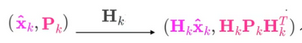
def project(self, mean, covariance):"""Project state distribution to measurement space.Parameters----------mean : ndarrayThe state's mean vector (8 dimensional array).covariance : ndarrayThe state's covariance matrix (8x8 dimensional).Returns-------(ndarray, ndarray)Returns the projected mean and covariance matrix of the given stateestimate."""std = [self._std_weight_position * mean[3], self._std_weight_position * mean[3], 1e-1,self._std_weight_position * mean[3]]innovation_cov = np.diag(np.square(std))mean = np.dot(self._update_mat, mean)covariance = np.linalg.multi_dot((self._update_mat, covariance, self._update_mat.T))return mean, covariance + innovation_cov

最后，結合觀測量，構建聯合高斯分布，更新狀態量。

def update(self, mean, covariance, measurement):"""Run Kalman filter correction step.Parameters----------mean : ndarrayThe predicted state's mean vector (8 dimensional).covariance : ndarrayThe state's covariance matrix (8x8 dimensional).measurement : ndarrayThe 4 dimensional measurement vector (x, y, a, h), where (x, y)is the center position, a the aspect ratio, and h the height of thebounding box.Returns-------(ndarray, ndarray)Returns the measurement-corrected state distribution."""projected_mean, projected_cov = self.project(mean, covariance)chol_factor, lower = scipy.linalg.cho_factor(projected_cov, lower=True, check_finite=False)kalman_gain = scipy.linalg.cho_solve((chol_factor, lower),np.dot(covariance, self._update_mat.T).T,check_finite=False).Tinnovation = measurement - projected_meannew_mean = mean + np.dot(innovation, kalman_gain.T)new_covariance = covariance - np.linalg.multi_dot((kalman_gain, projected_cov, kalman_gain.T))return new_mean, new_covariance