目錄
(一)數據建模
1.以數據預測為核心的建模
2.以數據聚類為核心的建模
(二)基本數據分析
1.Numpy
2. Pandas
3.實例
4.Matplotlib
資料自取:
鏈接: https://pan.baidu.com/s/1PROmz-2hR3VCTd6Eei6lFQ?pwd=y8ys 提取碼: y8ys
(一)數據建模
數據建模主要分為以數據預測為核心的建模與數據聚類為核心的建模
1.以數據預測為核心的建模
數據預測就是基于已有數據集,歸納出輸入變量和輸出變量之間的數量關系。數據預測可細分為回歸預測和分類預測。對數值型輸出變量的預測(對數值的預測)統稱為回歸預測。

對于自變量與因變量為非線性關系的情況:
擬合線性模型存在的潛在問題-CSDN博客
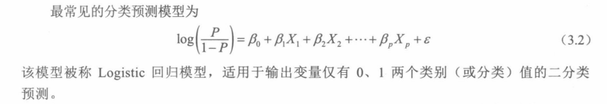
對分類型輸出變量的預測(對類別的預測)統稱為分類預測。如果輸出變量僅有兩個類別,則稱其為二分類預測。如果輸出變量有兩個以上的類別,則稱其為多分類預測。
2.以數據聚類為核心的建模
數據聚類就是發現數據重存在的更小的類,并通過小類刻畫和揭示數據的內在組織結構。例如根據相同性別,年齡,收入對顧客群進行細分。
數據聚類和數據預測中的分類問題:
聯系:數據聚類是給每個樣本觀測一個小類標簽;分類問題是給輸出變量一個分類值,本質也是給每個樣本觀測一個標簽。
區別:分類問題中的變量有輸入變量和輸出變量之分,且分類標簽(保存在輸出變量中,如空氣質量等級,顧客買或不買)的真實值是已知的;數據聚類中的變量沒有輸入變量和輸出變量之分,所有變量都將被視為聚類變量參與數據分析,且小類標簽(保存在聚類解變量中)的真實值是未知的。正是如此,數據聚類有著不同于數據分類的算法策略。?
注:除了以上兩種建模方式,還有關聯分析和模式診斷。關聯分析即探究不同事物之間的聯系。模式是一個數據集合,具有隨機和非常規性,例如下圖中,少量變動的數據即為模式。
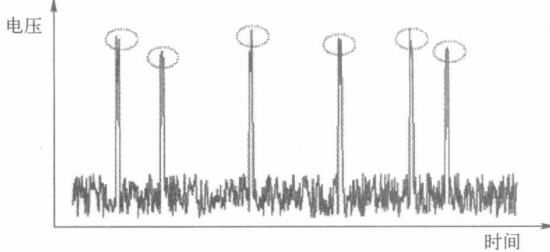
模式和統計學中的離群點不同:
盡管離群點與模式的數量都較少,且均表現出嚴重偏離數據全體的特征,但離群點通常由隨機因素所致。模式則不然,它具有非隨機性和潛在的形成機制。找到離群點的目的是剔除它們以消除對數據分析的影響,但模式很多時候就是人們關注的焦點,是不能剔除的。
(二)基本數據分析
1.Numpy
import numpy as np
data=np.array([1,2,3,4,5,6,7,8,9])
print('Numpy的1維數組:\n{0}'.format(data))
print('數據類型:%s'%data.dtype)
print('1維數組中各元素擴大10倍:\n{0}'.format(data*10))
print('訪問第2個元素:{0}'.format(data[1]))
data=np.array([[1,3,5,7,9],[2,4,6,8,10]])
print('Numpy的2維數組:\n{0}'.format(data))
print('訪問2維數組中第1行第2列元素:{0}'.format(data[0,1]))
print('訪問2維數組中第1行第2至4列元素:{0}'.format(data[0,1:4]))
print('訪問2維數組中第1行上的所有元素:{0}'.format(data[0,:]))#輸出:
Numpy的1維數組:
[1 2 3 4 5 6 7 8 9]
數據類型:int32
1維數組中各元素擴大10倍:
[10 20 30 40 50 60 70 80 90]
訪問第2個元素:2
Numpy的2維數組:
[[ 1  3  5  7  9][ 2  4  6  8 10]]
訪問2維數組中第1行第2列元素:3
訪問2維數組中第1行第2至4列元素:[3 5 7]
訪問2維數組中第1行上的所有元素:[1 3 5 7 9]data=[[1,2,3,4,5,6,7,8,9],['A','B','C','D','E','F','G','H','I']]
print('data是Python的列表(list):\n{0}'.format(data))
MyArray1=np.array(data)
print('MyArray1是Numpy的N維數組:\n%s\nMyarray1的形狀:%s'%(MyArray1,MyArray1.shape))#輸出
data是Python的列表(list):
[[1, 2, 3, 4, 5, 6, 7, 8, 9], ['A', 'B', 'C', 'D', 'E', 'F', 'G', 'H', 'I']]
MyArray1是Numpy的N維數組:
[['1' '2' '3' '4' '5' '6' '7' '8' '9']['A' 'B' 'C' 'D' 'E' 'F' 'G' 'H' 'I']]
Myarray1的形狀:(2, 9)MyArray2=np.arange(10)
print('MyArray2:\n{0}'.format(MyArray2))
print('MyArray2的基本描述統計量:\n均值:%f,標準差:%f,總和:%f,最大值:%f'%(MyArray2.mean(),MyArray2.std(),MyArray2.sum(),MyArray2.max()))
print('MyArray2的累計和:{0}'.format(MyArray2.cumsum()))
print('MyArray2開平方:{0}'.format(np.sqrt(MyArray2)))
np.random.seed(123) #復現隨機數
MyArray3=np.random.randn(10) #生成包含10個元素且服從標準正態分布的1維數組
print('MyArray3:\n{0}'.format(MyArray3))
print('MyArray3排序結果:\n{0}'.format(np.sort(MyArray3)))
print('MyArray3四舍五入到最近整數:\n{0}'.format(np.rint(MyArray3)))
print('MyArray3各元素的正負號:{0}'.format(np.sign(MyArray3)))
print('MyArray3各元素非負數的顯示"正",負數顯示"負":\n{0}'.format(np.where(MyArray3>0,'正','負')))
print('MyArray2+MyArray3的結果:\n{0}'.format(MyArray2+MyArray3))#輸出
MyArray2:
[0 1 2 3 4 5 6 7 8 9]
MyArray2的基本描述統計量:
均值:4.500000,標準差:2.872281,總和:45.000000,最大值:9.000000
MyArray2的累計和:[ 0  1  3  6 10 15 21 28 36 45]
MyArray2開平方:[0.         1.         1.41421356 1.73205081 2.         2.236067982.44948974 2.64575131 2.82842712 3.        ]
MyArray3:
[-1.0856306   0.99734545  0.2829785  -1.50629471 -0.57860025  1.65143654-2.42667924 -0.42891263  1.26593626 -0.8667404 ]
MyArray3排序結果:
[-2.42667924 -1.50629471 -1.0856306  -0.8667404  -0.57860025 -0.428912630.2829785   0.99734545  1.26593626  1.65143654]
MyArray3四舍五入到最近整數:
[-1.  1.  0. -2. -1.  2. -2. -0.  1. -1.]
MyArray3各元素的正負號:[-1.  1.  1. -1. -1.  1. -1. -1.  1. -1.]
MyArray3各元素非負數的顯示"正",負數顯示"負":
['負' '正' '正' '負' '負' '正' '負' '負' '正' '負']
MyArray2+MyArray3的結果:
[-1.0856306   1.99734545  2.2829785   1.49370529  3.42139975  6.651436543.57332076  6.57108737  9.26593626  8.1332596 ]np.random.seed(123)
#通過random.normal()生成2行5列的數組,服從均值5,標準差1的正態分布。再通過floor得到各元素最近的最大整數。
X=np.floor(np.random.normal(5,1,(2,5)))
#用eye函數聲稱單位矩陣
Y=np.eye(5)
print('X:\n{0}'.format(X))
print('Y:\n{0}'.format(Y))
print('X和Y的點積:\n{0}'.format(np.dot(X,Y)))#輸出
X:
[[3. 5. 5. 3. 4.][6. 2. 4. 6. 4.]]
Y:
[[1. 0. 0. 0. 0.][0. 1. 0. 0. 0.][0. 0. 1. 0. 0.][0. 0. 0. 1. 0.][0. 0. 0. 0. 1.]]
X和Y的點積:
[[3. 5. 5. 3. 4.][6. 2. 4. 6. 4.]]from numpy.linalg import inv,svd,eig,det
X=np.random.randn(5,5) #生成服從正態分布的5行5列矩陣
print(X)
#X的轉置與X相乘的結果保存在mat中
mat=X.T.dot(X)
print(mat)
print('矩陣mat的逆:\n{0}'.format(inv(mat)))
print('矩陣mat的行列式值:\n{0}'.format(det(mat)))
print('矩陣mat的特征值和特征向量:\n{0}'.format(eig(mat)))
print('對矩陣mat做奇異值分解:\n{0}'.format(svd(mat)))#輸出
[[-0.67888615 -0.09470897  1.49138963 -0.638902   -0.44398196][-0.43435128  2.20593008  2.18678609  1.0040539   0.3861864 ][ 0.73736858  1.49073203 -0.93583387  1.17582904 -1.25388067][-0.6377515   0.9071052  -1.4286807  -0.14006872 -0.8617549 ][-0.25561937 -2.79858911 -1.7715331  -0.69987723  0.92746243]]
[[ 1.6653281   0.3422329  -1.28839014  1.13288023 -0.47839144][ 0.3422329  15.75232012  6.94940128  5.8598402  -4.3525394 ][-1.28839014  6.94940128 13.06151953  1.58238781  0.94392314][ 1.13288023  5.8598402   1.58238781  3.30834132 -1.33134132][-0.47839144 -4.3525394   0.94392314 -1.33134132  3.52128471]]
矩陣mat的逆:
[[ 1.80352376  0.91697099 -0.13003481 -1.89987257  0.69500392][ 0.91697099  1.06125071 -0.33606314 -1.6733028   0.89378948][-0.13003481 -0.33606314  0.21904487  0.39759582 -0.34145532][-1.89987257 -1.6733028   0.39759582  3.24041446 -1.20785501][ 0.69500392  0.89378948 -0.34145532 -1.20785501  1.11805164]]
矩陣mat的行列式值:
105.54721777632028
矩陣mat的特征值和特征向量:
(array([23.58279263, 10.10645658,  2.29462217,  0.16661658,  1.1583058 ]), array([[-0.00179276, -0.18946636, -0.59452701, -0.46660531, -0.62683045],[ 0.77739059, -0.36419497,  0.09103298, -0.39431826,  0.31504284],[ 0.54092005,  0.77338945,  0.00371263,  0.10167527, -0.31451966],[ 0.27741393, -0.24680189, -0.58381349,  0.71576484,  0.09472503],[-0.16157864,  0.41523742, -0.54534269, -0.32270021,  0.63240505]]))
對矩陣mat做奇異值分解:
(array([[-0.00179276,  0.18946636,  0.59452701,  0.62683045,  0.46660531],[ 0.77739059,  0.36419497, -0.09103298, -0.31504284,  0.39431826],[ 0.54092005, -0.77338945, -0.00371263,  0.31451966, -0.10167527],[ 0.27741393,  0.24680189,  0.58381349, -0.09472503, -0.71576484],[-0.16157864, -0.41523742,  0.54534269, -0.63240505,  0.32270021]]), array([23.58279263, 10.10645658,  2.29462217,  1.1583058 ,  0.16661658]), array([[-0.00179276,  0.77739059,  0.54092005,  0.27741393, -0.16157864],[ 0.18946636,  0.36419497, -0.77338945,  0.24680189, -0.41523742],[ 0.59452701, -0.09103298, -0.00371263,  0.58381349,  0.54534269],[ 0.62683045, -0.31504284,  0.31451966, -0.09472503, -0.63240505],[ 0.46660531,  0.39431826, -0.10167527, -0.71576484,  0.32270021]]))
2. Pandas
序列(Series):
import numpy as np
import pandas as pd
from pandas import Series,DataFrame
data=Series([1,2,3,4,5,6,7,8,9],index=['ID1','ID2','ID3','ID4','ID5','ID6','ID7','ID8','ID9'])
print('序列中的值:\n{0}'.format(data.values))
print('序列中的索引:\n{0}'.format(data.index))
print('訪問序列的第1和第3上的值:\n{0}'.format(data[[0,2]]))
print('訪問序列索引為ID1和ID3上的值:\n{0}'.format(data[['ID1','ID3']]))
print('判斷ID1索引是否存在:%s;判斷ID10索引是否存在:%s'%('ID1' in data,'ID10' in data))import pandas as pd
from pandas import Series,DataFrame
data=pd.read_excel('北京市空氣質量數據.xlsx')
print('date的類型:{0}'.format(type(data)))
print('數據框的行索引:{0}'.format(data.index))
print('數據框的列名:{0}'.format(data.columns))
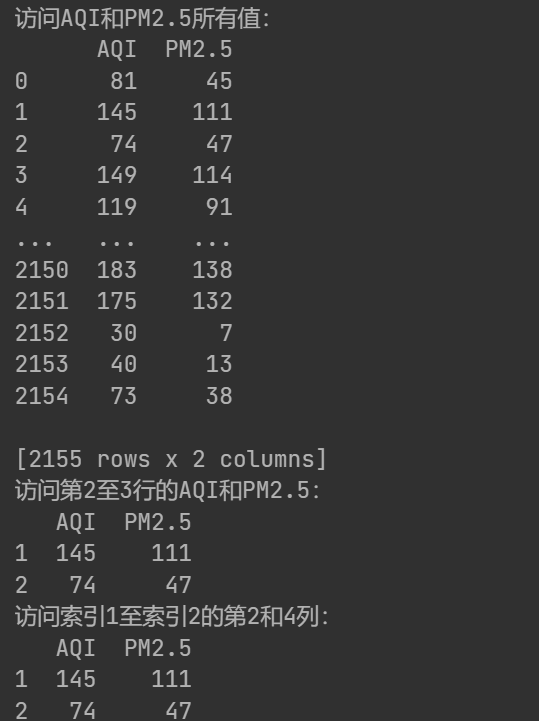
print('訪問AQI和PM2.5所有值:\n{0}'.format(data[['AQI','PM2.5']]))
print('訪問第2至3行的AQI和PM2.5:\n{0}'.format(data.loc[1:2,['AQI','PM2.5']]))
print('訪問索引1至索引2的第2和4列:\n{0}'.format(data.iloc[1:3,[1,3]]))
data.info()
注:
loc是基于標簽的索引,data.loc[1:2,]包含起始標簽和結束標簽,且是閉區間。表示選取標簽為1,2的行
iloc是基于位置的索引,data.iloc[1:3,]是左閉右開的,表示索引2,3
兩者打印結果相同:
數據框(DataFrame):
import numpy as np
import pandas as pd
from pandas import Series,DataFrame
df1=DataFrame({'key':['a','d','c','a','b','d','c'],'var1':range(7)})
df2=DataFrame({'key':['a','b','c','c'],'var2':[0,1,2,2]})
df=pd.merge(df1,df2,on='key',how='outer')
df.iloc[0,2]=np.NaN
df.iloc[5,1]=np.NaN
print('合并后的數據:\n{0}'.format(df))
df=df.drop_duplicates()
print('刪除重復數據行后的數據:\n{0}'.format(df))
print('判斷是否為缺失值:\n{0}'.format(df.isnull()))
print('判斷是否不為缺失值:\n{0}'.format(df.notnull()))
print('刪除缺失值后的數據:\n{0}'.format(df.dropna()))
#計算每列的均值
fill_value=df[['var1','var2']].apply(lambda x:x.mean())
#用均值填充
print('以均值替換缺失值:\n{0}'.format(df.fillna(fill_value)))
3.實例
import numpy as np
import pandas as pd
from pandas import Series,DataFramedata=pd.read_excel('北京市空氣質量數據.xlsx')
data=data.replace(0,np.NaN)
data['年']=data['日期'].apply(lambda x:x.year)
month=data['日期'].apply(lambda x:x.month)
quarter_month={'1':'一季度','2':'一季度','3':'一季度','4':'二季度','5':'二季度','6':'二季度','7':'三季度','8':'三季度','9':'三季度','10':'四季度','11':'四季度','12':'四季度'}
data['季度']=month.map(lambda x:quarter_month[str(x)])
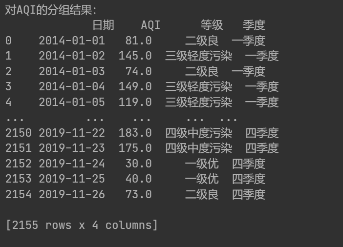
bins=[0,50,100,150,200,300,1000]
data['等級']=pd.cut(data['AQI'],bins,labels=['一級優','二級良','三級輕度污染','四級中度污染','五級重度污染','六級嚴重污染'])
print('對AQI的分組結果:\n{0}'.format(data[['日期','AQI','等級','季度']]))輸出:
print('各季度AQI和PM2.5的均值:\n{0}'.format(data.loc[:,['AQI','PM2.5']].groupby(data['季度']).mean()))
print('各季度AQI和PM2.5的描述統計量:\n',data.groupby(data['季度'])['AQI','PM2.5'].apply(lambda x:x.describe()))def top(df,n=10,column='AQI'):return df.sort_values(by=column,ascending=False)[:n]
print('空氣質量最差的5天:\n',top(data,n=5)[['日期','AQI','PM2.5','等級']])
print('各季度空氣質量最差的3天:\n',data.groupby(data['季度']).apply(lambda x:top(x,n=3)[['日期','AQI','PM2.5','等級']]))
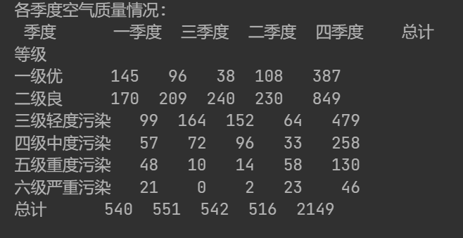
#crosstab可用于生成交叉表,行按等級分組,列按季度分組
print('各季度空氣質量情況:\n',pd.crosstab(data['等級'],data['季度'],margins=True,margins_name='總計',normalize=False))最后一行代碼輸出結果:
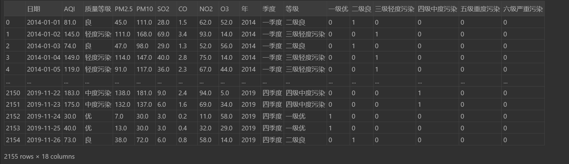
#用"0","1"表示改行是否屬于該等級
pd.get_dummies(data['等級'])
#并且合并到data中一起顯示
data.join(pd.get_dummies(data['等級']))
輸出:
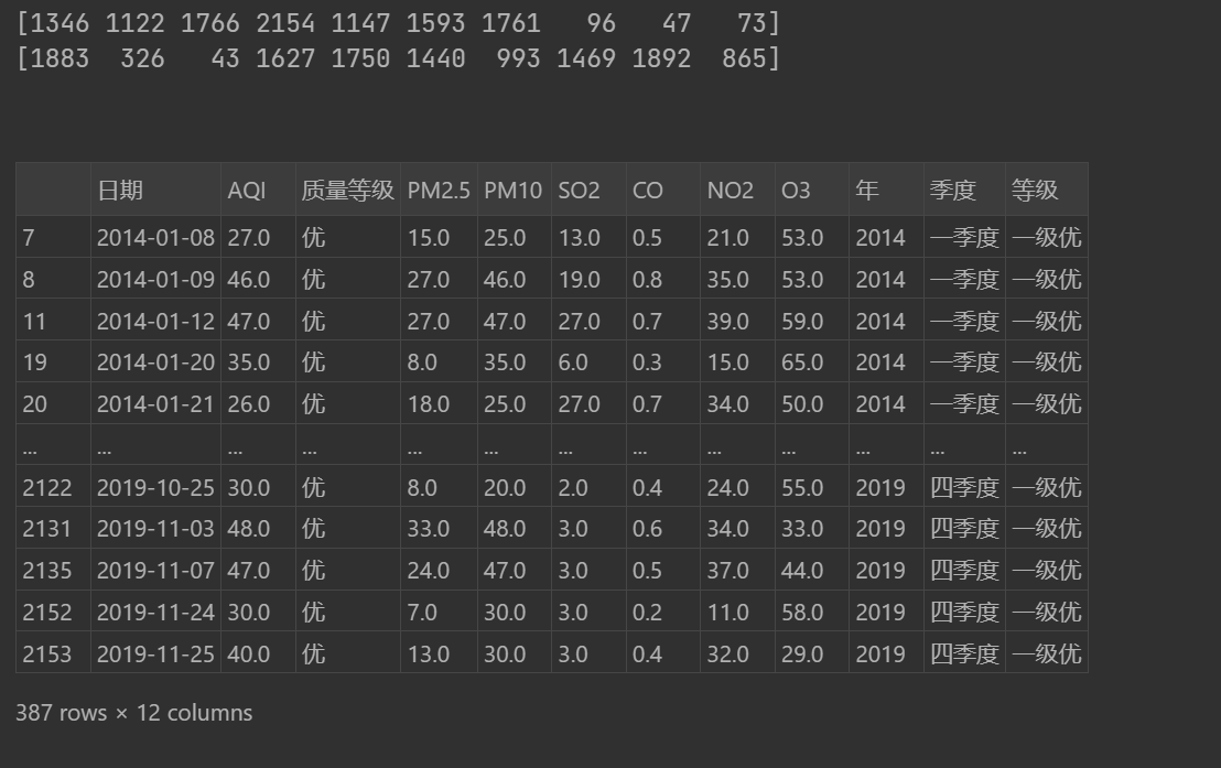
np.random.seed(123)
#np.random.randint(low, high, size),下限為low,上限為hign-1,打印個數為size
sampler=np.random.randint(0,len(data),10)
print(sampler)
#獲取data的總行數,截取前10個
sampler=np.random.permutation(len(data))[:10]
print(sampler)#基于隨機數獲取數據集
data.take(sampler)
#獲取"質量等級"為優的數據集
data.loc[data['質量等級']=='優',:]
輸出:
4.Matplotlib
import numpy as np
import pandas as pd
import matplotlib.pyplot as plt%matplotlib inline
plt.rcParams['font.sans-serif']=['SimHei']  #解決中文顯示亂碼問題
plt.rcParams['axes.unicode_minus']=Falsedata=pd.read_excel('北京市空氣質量數據.xlsx')
data=data.replace(0,np.NaN)plt.figure(figsize=(10,5))
plt.plot(data['AQI'],color='black',linestyle='-',linewidth=0.5)
plt.axhline(y=data['AQI'].mean(),color='red', linestyle='-',linewidth=0.5,label='AQI總平均值')
data['年']=data['日期'].apply(lambda x:x.year)
AQI_mean=data['AQI'].groupby(data['年']).mean().values
year=['2014年','2015年','2016年','2017年','2018年','2019年']
col=['red','blue','green','yellow','purple','brown']
for i in range(6):plt.axhline(y=AQI_mean[i],color=col[i], linestyle='--',linewidth=0.5,label=year[i])
plt.title('2014年至2019年AQI時間序列折線圖')
plt.xlabel('年份')
plt.ylabel('AQI')
plt.xlim(xmax=len(data), xmin=1)
plt.ylim(ymax=data['AQI'].max(),ymin=1)
plt.yticks([data['AQI'].mean()],['AQI平均值'])
plt.xticks([1,365,365*2,365*3,365*4,365*5],['2014','2015','2016','2017','2018','2019'])
plt.legend(loc='best')
plt.text(x=list(data['AQI']).index(data['AQI'].max()),y=data['AQI'].max()-20,s='空氣質量最差日',color='red')
plt.show()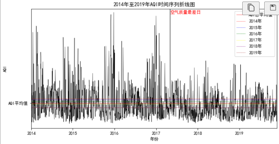
import warnings
warnings.filterwarnings(action = 'ignore')
plt.figure(figsize=(10,5))
#圖表分為2行2列,選取第1個位置
plt.subplot(2,2,1)
plt.plot(AQI_mean,color='black',linestyle='-',linewidth=0.5)
plt.title('各年AQI均值折線圖')
#[0,1,2,3,4..]是實際刻度,['2014','2015'..]是對應標簽
plt.xticks([0,1,2,3,4,5,6],['2014','2015','2016','2017','2018','2019'])
plt.subplot(2,2,2)
plt.hist(data['AQI'],bins=20)
plt.title('AQI直方圖')
plt.subplot(2,2,3)
#行為PM2.5,列為AQI
plt.scatter(data['PM2.5'],data['AQI'],s=0.5,c='green',marker='.')
plt.title('PM2.5與AQI散點圖')
plt.xlabel('PM2.5')
plt.ylabel('AQI')
plt.subplot(2,2,4)
tmp=pd.value_counts(data['質量等級'],sort=False)  #等同:tmp=data['質量等級'].value_counts(),統計各等級出現的次數
share=tmp/sum(tmp)
labels=tmp.index
explode = [0, 0.2, 0, 0, 0,0.2,0]
plt.pie(share, explode = explode,labels = labels, autopct = '%3.1f%%',startangle = 180, shadow = True)
plt.title('空氣質量整體情況的餅圖')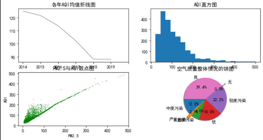
以下代碼通過axes[0,0]直接定位子圖,比plt.subplot容易維護,例如,如果刪除第2個子圖,則(2,2,3)--->(2,2,2),(2,2,4)--->(2,2,3)。
fig,axes=plt.subplots(nrows=2,ncols=2,figsize=(10,5))
axes[0,0].plot(AQI_mean,color='black',linestyle='-',linewidth=0.5)
axes[0,0].set_title('各年AQI均值折線圖')
axes[0,0].set_xticks([0,1,2,3,4,5,6])
axes[0,0].set_xticklabels(['2014','2015','2016','2017','2018','2019'])
axes[0,1].hist(data['AQI'],bins=20)
axes[0,1].set_title('AQI直方圖')
axes[1,0].scatter(data['PM2.5'],data['AQI'],s=0.5,c='green',marker='.')
axes[1,0].set_title('PM2.5與AQI散點圖')
axes[1,0].set_xlabel('PM2.5')
axes[1,0].set_ylabel('AQI')
axes[1,1].pie(share, explode = explode,labels = labels, autopct = '%3.1f%%',startangle = 180, shadow = True)
axes[1,1].set_title('空氣質量整體情況的餅圖')
fig.subplots_adjust(hspace=0.5)#調整垂直間距
fig.subplots_adjust(wspace=0.5)#調整水平間距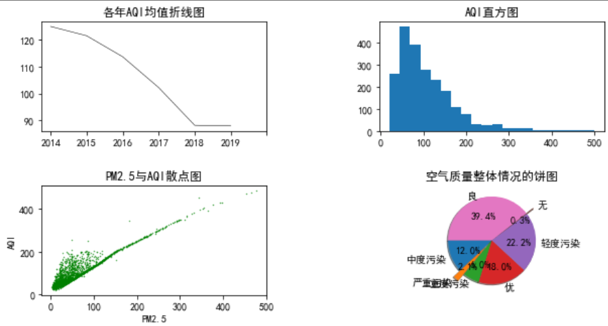


![[硬件電路-148]:數字電路 - 什么是CMOS電平、TTL電平?還有哪些其他電平標準?發展歷史?](http://pic.xiahunao.cn/[硬件電路-148]:數字電路 - 什么是CMOS電平、TTL電平?還有哪些其他電平標準?發展歷史?)
 --(前端篇 2)--)


)


常用管理SQL命令(3))
