5月14日復盤

二、BiLSTM

1. 概述

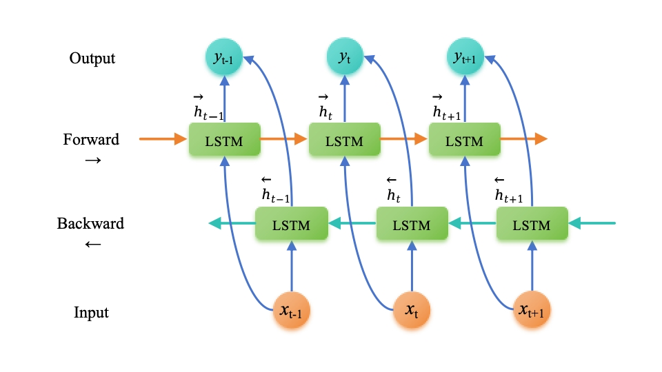
雙向長短期記憶網絡（Bi-directional Long Short-Term Memory，BiLSTM）是一種擴展自長短期記憶網絡（LSTM）的結構，旨在解決傳統 LSTM 模型只能考慮到過去信息的問題。BiLSTM 在每個時間步同時考慮了過去和未來的信息，從而更好地捕捉了序列數據中的雙向上下文關系。

BiLSTM 的創新點在于引入了兩個獨立的 LSTM 層，一個按正向順序處理輸入序列，另一個按逆向順序處理輸入序列。這樣，每個時間步的輸出就包含了當前時間步之前和之后的信息，進而使得模型能夠更好地理解序列數據中的語義和上下文關系。

• 正向傳遞: 輸入序列按照時間順序被輸入到第一個LSTM層。每個時間步的輸出都會被計算并保留下來。

• 反向傳遞: 輸入序列按照時間的逆序（即先輸入最后一個元素）被輸入到第二個LSTM層。與正向傳遞類似，每個時間步的輸出都會被計算并保留下來。

• 合并輸出: 在每個時間步，將兩個LSTM層的輸出通過某種方式合并（如拼接或加和）以得到最終的輸出。

2. BILSTM模型應用背景

命名體識別

標注集

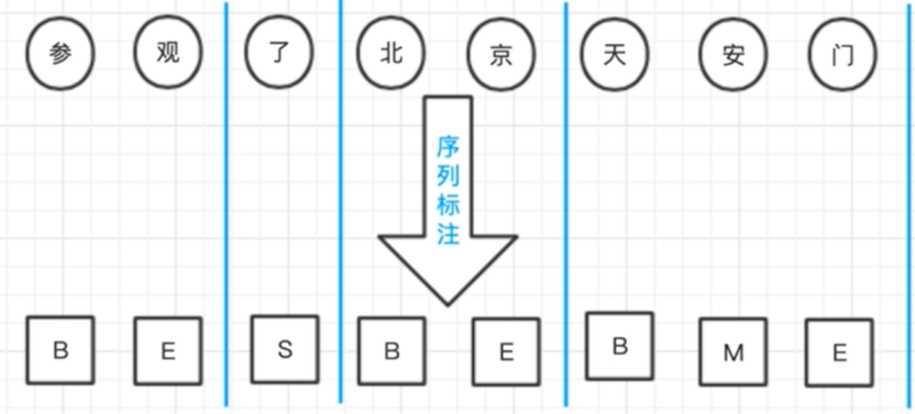
BMES標注集

分詞的標注集并非只有一種，舉例中文分詞的情況，漢子作為詞語開始Begin，結束End,中間Middle，單字Single，這四種情況就可以囊括所有的分詞情況。于是就有了BMES標注集，這樣的標注集在命名實體識別任務中也非常常見。

詞性標注

在序列標注問題中單詞序列就是x，詞性序列就是y，當前詞詞性的判定需要綜合考慮前后單詞的詞性。而標注集最著名的就是863標注集和北大標注集。

3. 代碼實現

原生代碼

import numpy as npdef sigmoid(x):return 1 / (1 + np.exp(-x))def tanh(x):return np.tanh(x)class GRU:def __init__(self, input_size, hidden_size, output_size):self.input_size = input_sizeself.hidden_size = hidden_sizeself.output_size = output_size#權重矩陣和偏置self.W_z = np.random.randn(hidden_size + input_size, hidden_size)self.b_z = np.zeros((hidden_size,))self.W_r = np.random.randn(hidden_size + input_size, hidden_size)self.b_r = np.zeros((hidden_size,))# ht候選self.W = np.random.randn(hidden_size + input_size, hidden_size)self.b = np.zeros((hidden_size,))def forward(self, x, h_last):""":param x: [s,dim]:param h_last::return:"""# 初始化狀態h_prev = np.zeros((self.hidden_size,))h_all = []for i in range(x.shape[0]):x_t = x[i]x_t_h_prev = np.concatenate((x_t, h_prev), axis=0)r_t = sigmoid(np.dot(x_t_h_prev, self.W_r) + self.b_r)z_t = sigmoid(np.dot(x_t_h_prev, self.W_z) + self.b_z)# h_prev = r_t * h_prevh_t_input = np.concatenate((x_t, h_prev * r_t), axis=0)h_t_candidate = tanh(np.dot(h_t_input, self.W) + self.b)h_t = (1 - z_t) * h_prev + z_t * h_t_candidateh_all.append(h_t)return h_allif __name__ == '__main__':gru = GRU(input_size=2, hidden_size=5, output_size=1)x = np.random.randn(3 , 2)h_last = np.zeros((3,))h_all = gru.forward(x, h_last)print(h_all)

# ---------------------------------------------------------------------------
import numpy as np# 創建一個包含兩個二維數組的列表
inputs = [np.array([[0.1], [0.2], [0.3]]), np.array([[0.4], [0.5], [0.6]])]# 使用 numpy 庫中的 np.stack 函數。這會將輸入的二維數組堆疊在一起，從而形成一個新的三維數組
inputs_3d = np.stack(inputs)# 將三維數組轉換為列表
list_from_3d_array = inputs_3d.tolist()print(list_from_3d_array)

Pytorch

import torch
import torch.nn as nn# 模型參數設置
batch_size = 10
sen_len = 6
hidden_size = 8input_size = 3
output_size = hidden_size * 2  # 類別是隱藏層大小的兩倍# 初始化隱藏層狀態
h_prev = torch.zeros(1, batch_size, hidden_size)# RNN調用
model = nn.GRU(input_size, hidden_size, batch_first=True)
fc = nn.Linear(hidden_size, output_size)  # 全連接層用于分類# 初始化數據
x = torch.randn(10, 6, 3)out, h_next = model(x, h_prev)
# 對每個時間步的輸出進行分類
out = out.contiguous().view(-1, hidden_size)  # 調整形狀為 (batch_size * sen_len, hidden_size)
out = fc(out)
out = out.view(batch_size, sen_len, output_size)  # 調整回 (batch_size, sen_len, output_size)print("多對多輸出:")
print(out.shape)
print(out)
print(h_next.shape)
print(h_next)out, h_next = model(x, h_prev)
# 只對最后一個時間步的輸出進行分類
final_out = h_next.squeeze(0)  # 移除多余的維度，得到 (batch_size, hidden_size)
final_out = fc(final_out)print("\n多對一輸出:")
print(final_out.shape)
print(final_out)
print(h_next.shape)
print(h_next)