目錄
- 一、歷史
- 二、精髓思想
- 三、案例與代碼實現
一、歷史
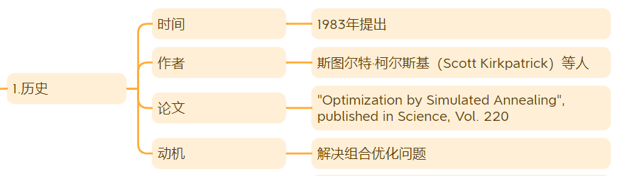
- 問:誰在什么時候提出模擬退火?
- 答:模擬退火算法(Simulated Annealing,SA)是由斯圖爾特·柯爾斯基(Scott Kirkpatrick) 等人在 1983年 提出的。
- 論文:“Optimization by Simulated Annealing”, published in Science, Vol. 220
- 動機:解決組合優化問題
二、精髓思想
- 精髓就兩字:退火!
- 解釋:字面意思就是模擬打鐵的退火過程,剛開始打鐵吧溫度比較高,鐵燒的紅紅的容易打出各種形狀,隨著時間變長,溫度逐漸冷卻下來,鐵更硬了,形狀大方向基本確定。
不禁感嘆,以前的物理學家、數學家靈感來源都是自然現象!

總結下來其實就3個step:
- 拿一塊鐵過來淬火
- 打一次看看如何
- 給我打到定型
三、案例與代碼實現
-
題干:
6艘船靠3個港口,已知達到時間arrival和卸貨時長handling,求最優停靠方案,即等待時長最短。 -
數據:
ships = {'S1': {'arrival': 0.1, 'handling': 4},'S2': {'arrival': 2.1, 'handling': 3},'S3': {'arrival': 4.2, 'handling': 2},'S4': {'arrival': 6.3, 'handling': 3},'S5': {'arrival': 5.5, 'handling': 2},'S6': {'arrival': 3.9, 'handling': 4},'S7': {'arrival': 3.7, 'handling': 4},'S8': {'arrival': 3.4, 'handling': 4},
}
- 實現:
step1:拿一塊鐵過來淬火
# 隨機初始化一塊鐵(船舶調度順序)
initial_order = list(ships.keys()) # 船舶原始順序['S1', 'S2', 'S3', 'S4', 'S5', 'S6', 'S7', 'S8']
random.shuffle(initial_order)	#	打亂順序 ,可能是['S2', 'S7', 'S6', 'S5', 'S1', 'S3', 'S4', 'S8']
- step2:打一次看看如何
首先,先評價一下原始模樣如何?用等待時間作為衡量,如下:
current_cost = evaluate(current)
NUM_BERTHS = 3  # 泊位數量
# 評價函數:計算某個調度順序的總等待時間
def evaluate(order):berth_times = [0] * NUM_BERTHStotal_wait = 0for ship_id in order:arrival = ships[ship_id]['arrival']handling = ships[ship_id]['handling']# 找到最早可用泊位berth_index = min(range(NUM_BERTHS), key=lambda i: max(arrival, berth_times[i]))# start_time = 開始卸貨時間 = max(到達時間, 泊位可用時間)。# 解釋:要卸貨的話,船先到達了沒有泊位可用也得等,反之,有空泊位了船還沒到也得等。start_time = max(arrival, berth_times[berth_index])wait_time = start_time - arrivaltotal_wait += wait_timeberth_times[berth_index] = start_time + handlingreturn total_wait
然后,開始下錘子了(稱之為擾動)
# 生成鄰域解(隨機交換兩艘船順序)
def neighbor(order):new_order = order.copy()i, j = random.sample(range(len(order)), 2)new_order[i], new_order[j] = new_order[j], new_order[i]return new_order
緊接著,評估下現在模樣和上一次區別,如下:
new = neighbor(current)
new_cost = evaluate(new)
delta = new_cost - current_cost	# 擾動之后的區別
最后,做決定是接著現在模樣往下繼續打,還是恢復回原來模樣
# 情況1:delta < 0 說明等待時間變短了呀,打鐵打得更好了,欣然接受。
# 情況2:delta >= 0 說明等待時間變長了,糟糕打偏了,不過沒關系,這是藝術啊!不完美也是一種美!看心情決定~
# 于是有了 random.random() < math.exp(-delta / T)這一項
# 解釋:random.random()就是一個隨機值(類比于當時心情),值域范圍[0.0, 1.0)
# math.exp(-delta / T)和delta、T有關系,這么來看吧,假設現在超級無敵高溫,那么-delta / T趨于0,那么math.exp(-delta / T)趨于1,說明有很大概率接受比較差的解。假設現在溫度快降到0了,那么-delta / T趨于負無窮,那么math.exp(-delta / T)趨于0,說明有極小概率接受比較差的解。
if delta < 0 or random.random() < math.exp(-delta / T):current = newcurrent_cost = new_cost
- step3:給我打到定型
循環的過程,就是往復step2的過程,持續下去直到定型,如下:
# 模擬退火主過程
# 初始順序:initial_order, 溫度:T=100.0, 冷卻率:cooling_rate=0.95, 最低溫度:T_min=1e-3
def simulated_annealing(initial_order, T=100.0, cooling_rate=0.95, T_min=1e-3):current = initial_ordercurrent_cost = evaluate(current)best = currentbest_cost = current_costwhile T > T_min:for _ in range(100):  # 每個溫度嘗試多次擾動new = neighbor(current)new_cost = evaluate(new)delta = new_cost - current_costif delta < 0 or random.random() < math.exp(-delta / T):current = newcurrent_cost = new_costif current_cost < best_cost:best = currentbest_cost = current_costT *= cooling_rate  # 降溫return best, best_cost


Swift安裝)


)


)


