機器學習【三】SVM

? ? 本文系統介紹了支持向量機(SVM)的理論與實踐。理論部分首先區分了線性可分與不可分問題，闡述了SVM通過尋找最優超平面實現分類的核心思想，包括支持向量、間隔最大化等關鍵概念。詳細講解了硬間隔與軟間隔SVM的數學原理，以及核函數(線性核、多項式核、RBF核)在非線性問題中的應用。實踐部分通過Python代碼演示了SVM在不同場景下的應用：線性可分數據分類、參數C的調節效果、非線性數據分類中核函數的選擇比較，并以信用卡欺詐檢測為例，展示了網格搜索調參和模型評估的完整流程。最后總結了SVM在小樣本、高維數據中的優勢及其參數敏感的局限性。。

1 線性可分與線性不可分

????????在分類任務中（二分類為典型代表），我們需要找到一個模型（或稱為決策邊界）來區分不同類別的數據點。

??線性可分：?? 如果存在一個??線性??的決策邊界（在特征空間中表現為一條直線、一個平面或一個超平面），能夠完美地將屬于不同類別的數據點分隔開來（即所有正類樣本在邊界的一側，所有負類樣本在另一側，沒有樣本被錯誤分類），那么我們稱這個數據集在該特征空間中是??線性可分??的。
??核心：?? 分類任務可以通過一個簡單的線性模型（如線性函數）100%準確完成。

??線性不可分：?? 如果不存在任何一條直線、一個平面或一個超平面能夠完美地將不同類別的數據點區分開來（即任何線性邊界都會錯誤地分類至少一部分樣本），那么我們稱這個數據集在該特征空間中是??線性不可分??的。
??核心：?? 無法僅用一個線性模型來獲得完美的分類精度。需要一個更復雜的（通常是??非線性??的）模型來處理數據的分布。

????????我們可以想象一張紙上有兩種顏色的豆子，線性可分是可以用一支筆劃一條直線分開兩種顏色豆子。而線性不可分就是兩種顏色豆子混雜在一起，無法劃一條直線完全分開。

? ? ? ? ?而支持向量機（SVM）要解決的就是什么樣的決策邊界是最好的？特征數據本身如果就很難分，該怎么辦？計算復雜度怎么樣？能實際應用嘛？

2 SVM基本概念

支持向量機（SVM）是一類按監督學習方式對數進行二元分類的廣義線性分類器

2.1 核心思想

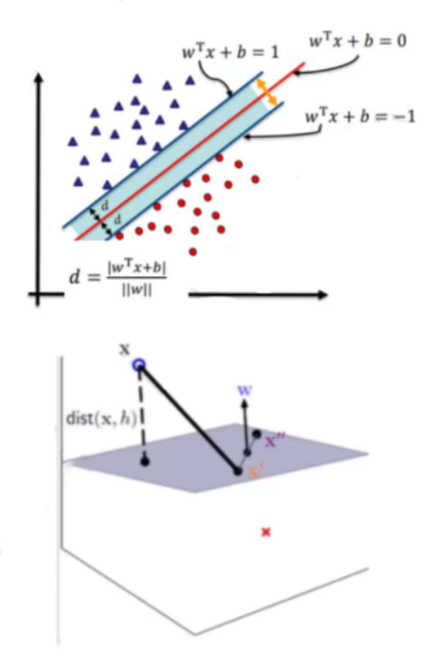
? SVM的目標是找到一個??決策超平面??（Decision Hyperplane），不僅正確分類數據，還要確保該平面??距離最近的數據點最遠??。

? 假設我們是要在兩國爭議地帶劃界，需要滿足：公平性??：邊界離兩國最近的村莊距離相等（分類準確）。安全性??：邊界離兩國領土盡可能遠（最大化間隔），這就是SVM的追求??。

2.2 關鍵組成

術語	數學意義	生活比喻
??超平面??	$w\cdot x+b=0$	劃界的“墻”
??支持向量??	離超平面最近的樣本點	邊界上的“爭議村莊”
??間隔??	$\frac{2}{\|\|W\|\|}$	邊界到村莊的安全距離

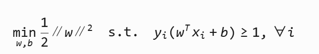
3 SVM距離定義

這些理論和內容已經有完整的數學體系不進行深入的學習和介紹。知其然即可

超平面可以用一個線性方程來描述：? $W^{_{T}}x+b=0$ ?。在二維空間點（x,y）到直線Ax + By + C = 0的距離為： $\tfrac{Ax+By+C}{\sqrt{A^{2}+B^{2}}}$ ?擴展到n維空間后點x = （x1,x2,...,xn）到直線? $W^{_{T}}x+b=0$ ?的距離為：? $\left \| w \right \| = \sqrt{w_{1}^{2} + ... + w_{n}^{2}}$ ???? $\frac{1}{\left \| W \right \|}|W^{_{T}}x+b|$

4 SVM決策面

根據支持向量的定義，我們知道，支持向量到超平面的距離為d。其他點到超面的距離大于d，我們暫且令d為1。于是我們得到：

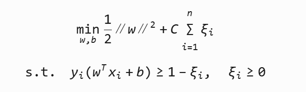
$\left\{\begin{matrix} \frac{W^{_{T}}x+b }{|w|} \geqslant d& y = 1\\ \frac{W^{_{T}}x+b }{|w|} \leq -d& y =- 1 \end{matrix}\right.$

5 SVM優化目標

使用的拉格朗日乘子算法條件進行了優化

6 SVM軟間隔

??由于噪音數據或輕微線性不可分導致找不到完美分隔。因此引入松弛變量?ξi?，允許少量錯誤。

?C為懲罰參數，C越大，對分類的懲罰就越大。

7 SVM核變換

核函數將樣本從原始空間映射到一個更高維的特質空間中，使得樣本在新的空間中線性可分

核函數	公式	特點
線性核	xiT?xj?	不進行高維映射
多項式核	(γxiT?xj?+r)d	可調階數?d
RBF核	exp(?γ∥xi??xj?∥2)	最常用，非線性強

?8 練習使用

上述內容基本都是理論和實際公式以及推導的一些內容，還是直接使用代碼使用來強化使用和參數調整的學習

線性可分的數據

import numpy as np
import matplotlib.pyplot as plt
from sklearn.svm import SVC# ===== 1. 數據準備 =====
X = np.array([[1, 2],  # 負類點1[2, 3],  # 負類點2[2, 1],  # 正類點1[3, 2]   # 正類點2
])
y = np.array([-1, -1, 1, 1])  # 前兩個負類，后兩個正類# ===== 2. 模型訓練 =====
model = SVC(kernel='linear', C=1000)
model.fit(X, y)# ===== 3. 可視化修復 =====
plt.figure(figsize=(8, 6))# 先繪制數據點 (先創建坐標系)
plt.scatter(X[:, 0], X[:, 1], c=y, s=100, cmap=plt.cm.Paired,edgecolor='k', marker='o')# 設置坐標軸范圍 (顯式設定確保邊界完整)
plt.xlim(0.5, 3.5)  # 覆蓋所有X值
plt.ylim(0.5, 3.5)  # 覆蓋所有Y值# 生成網格點 (基于當前坐標系范圍)
ax = plt.gca()
xlim = ax.get_xlim()
ylim = ax.get_ylim()xx = np.linspace(xlim[0], xlim[1], 100)
yy = np.linspace(ylim[0], ylim[1], 100)
YY, XX = np.meshgrid(yy, xx)
xy = np.vstack([XX.ravel(), YY.ravel()]).T# 計算決策函數值
Z = model.decision_function(xy).reshape(XX.shape)# 關鍵修復：使用contourf填充背景展示決策效果
# 填充決策區域（更直觀顯示分類）
plt.contourf(XX, YY, Z, levels=[-np.inf, 0, np.inf],alpha=0.3, colors=['blue', 'orange'])# 繪制決策邊界和間隔線（三種線型區分）
plt.contour(XX, YY, Z, colors='k',levels=[-1, 0, 1],linestyles=[':', '-', ':'],linewidths=[1, 2, 1])# 標記支持向量（紅框突出顯示）
plt.scatter(model.support_vectors_[:, 0],model.support_vectors_[:, 1],s=200, facecolors='none',edgecolors='red', linewidths=2,label='Support Vectors')# 添加決策邊界公式（數學展示）
w = model.coef_[0]
b = model.intercept_[0]
boundary_text = f'Decision Boundary: {w[0]:.1f}x + {w[1]:.1f}y + {b:.1f} = 0'
plt.text(1.0, 3.2, boundary_text, fontsize=12, bbox=dict(facecolor='white', alpha=0.7))# 添加間隔線說明
plt.text(0.6, 1.0, 'Margin Boundary', fontsize=10, color='purple', rotation=50)# 添加標題和標簽
plt.title(f"Linear SVM (C={model.C})", fontsize=14)
plt.xlabel("Feature 1", fontsize=12)
plt.ylabel("Feature 2", fontsize=12)
plt.grid(True, linestyle='--', alpha=0.4)
plt.legend()plt.tight_layout()
plt.show()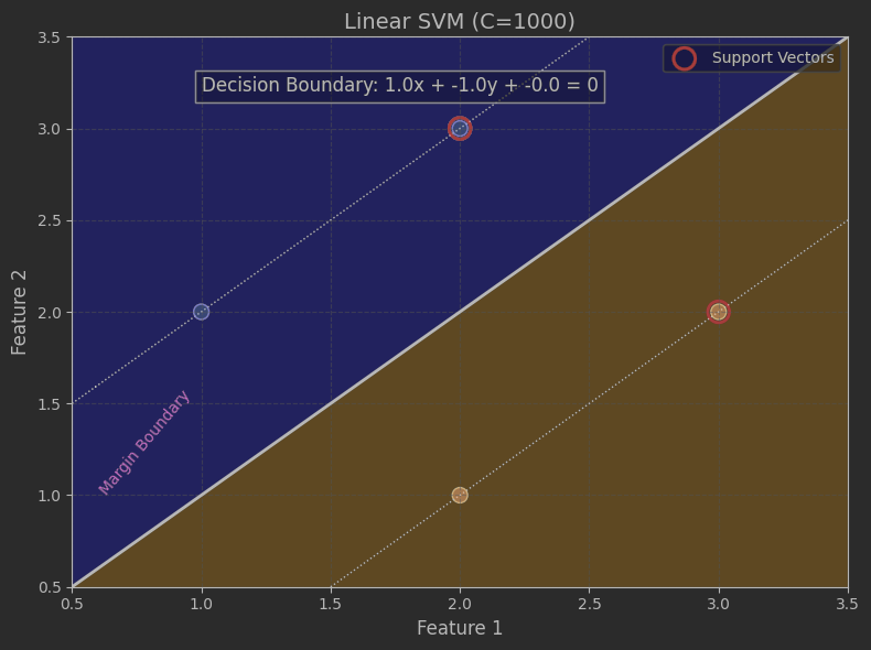

SVM調整

import numpy as np
import matplotlib.pyplot as plt
from sklearn.svm import SVC# 統一數據集
X = np.array([[1, 2], [2, 3], [2, 1], [3, 2]
])
y = np.array([-1, -1, 1, 1])# 確定全局坐標范圍（所有子圖統一）
x_min, x_max = 0.5, 3.5
y_min, y_max = 0.5, 3.5# 創建高密度網格（固定范圍）
xx = np.linspace(x_min, x_max, 200)
yy = np.linspace(y_min, y_max, 200)
XX, YY = np.meshgrid(xx, yy)
grid_points = np.c_[XX.ravel(), YY.ravel()]# 不同C值對比實驗
C_values = [0.01, 1, 100]
plt.figure(figsize=(15, 5))for i, C_val in enumerate(C_values):# 訓練不同C值的模型model = SVC(kernel='linear', C=C_val)model.fit(X, y)# 計算決策函數值Z = model.decision_function(grid_points).reshape(XX.shape)# 繪制子圖ax = plt.subplot(1, 3, i+1)# 繪制決策區域背景（輔助觀察）ax.pcolormesh(XX, YY, np.sign(Z), cmap=plt.cm.Paired, alpha=0.2)# 繪制決策邊界（3條線）ax.contour(XX, YY, Z, colors='k',levels=[-1, 0, 1],linestyles=[':', '-', ':'],linewidths=[1, 2, 1])# 標記支持向量ax.scatter(model.support_vectors_[:, 0], model.support_vectors_[:, 1],s=150, facecolors='none', edgecolors='red',linewidths=1.5, label='Support Vectors')# 繪制數據點ax.scatter(X[:, 0], X[:, 1], c=y, s=100, cmap=plt.cm.Paired,edgecolors='k', zorder=10)# 統一范圍設置ax.set_xlim(x_min, x_max)ax.set_ylim(y_min, y_max)# 添加標題和網格ax.set_title(f"C = {C_val}\nSupport Vectors: {len(model.support_vectors_)}")ax.grid(True, linestyle='--', alpha=0.3)# 添加決策邊界公式w = model.coef_[0]b = model.intercept_[0]equation = f"{w[0]:.2f}x + {w[1]:.2f}y + {b:.2f} = 0"ax.text(1.0, 3.3, equation, fontsize=10,bbox=dict(facecolor='white', alpha=0.7))# 添加主標題
plt.suptitle("Effect of C Parameter in Linear SVM", fontsize=16, y=0.98)
plt.tight_layout()
plt.show()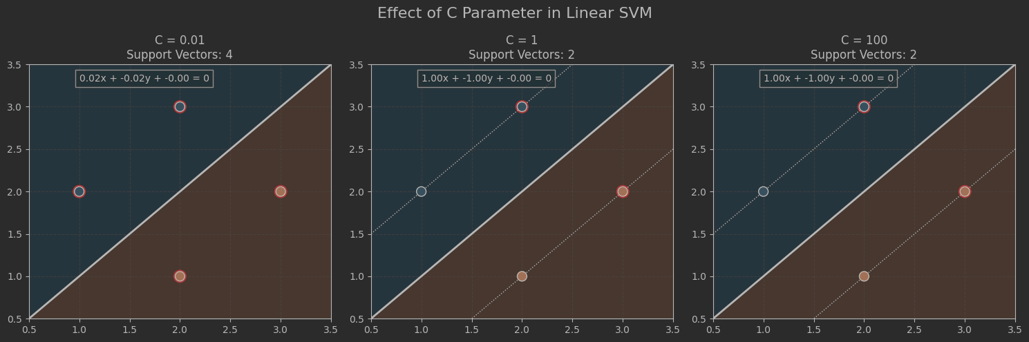

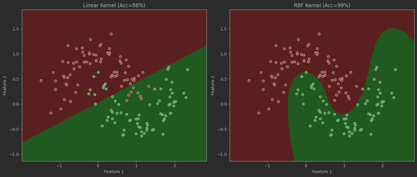
非線性數據

# 非線性數據分類
from sklearn.datasets import make_moons
from sklearn.model_selection import train_test_split
import matplotlib.pyplot as plt
from matplotlib.colors import ListedColormap# ===== 1. 生成非線性數據 =====
'''
參數說明：
- noise=0.2：20%的噪聲（控制數據混雜度）
- random_state=42：固定隨機種子
'''
X, y = make_moons(n_samples=500, noise=0.2, random_state=42)# ===== 2. 數據分割 =====
X_train, X_test, y_train, y_test = train_test_split(X, y,test_size=0.3,      # 30%測試集random_state=42
)# ===== 3. 線性核表現 =====
linear_svm = SVC(kernel='linear', C=0.1)
linear_svm.fit(X_train, y_train)
lin_score = linear_svm.score(X_test, y_test)
print(f"Linear SVM Accuracy: {lin_score:.2%}")  # ~55-65%# ===== 4. RBF核表現 =====
rbf_svm = SVC(kernel='rbf', gamma=1, C=10)
rbf_svm.fit(X_train, y_train)
rbf_score = rbf_svm.score(X_test, y_test)
print(f"RBF SVM Accuracy: {rbf_score:.2%}")  # ~90-95%# ===== 5. 可視化函數 =====
def plot_decision_boundary(model, X, y, title):# 生成網格h = 0.02  # 網格步長x_min, x_max = X[:, 0].min()-0.5, X[:, 0].max()+0.5y_min, y_max = X[:, 1].min()-0.5, X[:, 1].max()+0.5xx, yy = np.meshgrid(np.arange(x_min, x_max, h),np.arange(y_min, y_max, h))# 預測網格分類Z = model.predict(np.c_[xx.ravel(), yy.ravel()])Z = Z.reshape(xx.shape)# 創建配色cmap_light = ListedColormap(['#FFAAAA', '#AAFFAA'])cmap_bold = ListedColormap(['#FF0000', '#00FF00'])# 繪制決策區域plt.pcolormesh(xx, yy, Z, cmap=cmap_light, alpha=0.8)# 繪制數據點plt.scatter(X[:, 0], X[:, 1], c=y,cmap=cmap_bold, s=30, edgecolor='k')plt.xlim(xx.min(), xx.max())plt.ylim(yy.min(), yy.max())plt.title(title)plt.xlabel("Feature 1")plt.ylabel("Feature 2")# ===== 6. 對比可視化 =====
plt.figure(figsize=(14, 6))plt.subplot(121)
plot_decision_boundary(linear_svm, X_test, y_test,f"Linear Kernel (Acc={lin_score:.0%})")plt.subplot(122)
plot_decision_boundary(rbf_svm, X_test, y_test,f"RBF Kernel (Acc={rbf_score:.0%})")plt.tight_layout()
plt.show()

SVM優化

# 參數調整
# RBF核參數網格分析
plt.figure(figsize=(16, 12))
C_values = [0.1, 1, 10, 100]
gamma_values = [0.1, 1, 10, 100]for i, C in enumerate(C_values):for j, gamma in enumerate(gamma_values):# 訓練模型model = SVC(kernel='rbf', C=C, gamma=gamma)model.fit(X_train, y_train)acc = model.score(X_test, y_test)# 繪制子圖plt.subplot(4, 4, i*4 + j+1)plot_decision_boundary(model, X_test, y_test,f"C={C}, γ={gamma}\nAcc={acc:.0%}")plt.grid(False)plt.tight_layout()
plt.suptitle("RBF Kernel Parameter Effects", y=1.02, fontsize=16)
plt.show()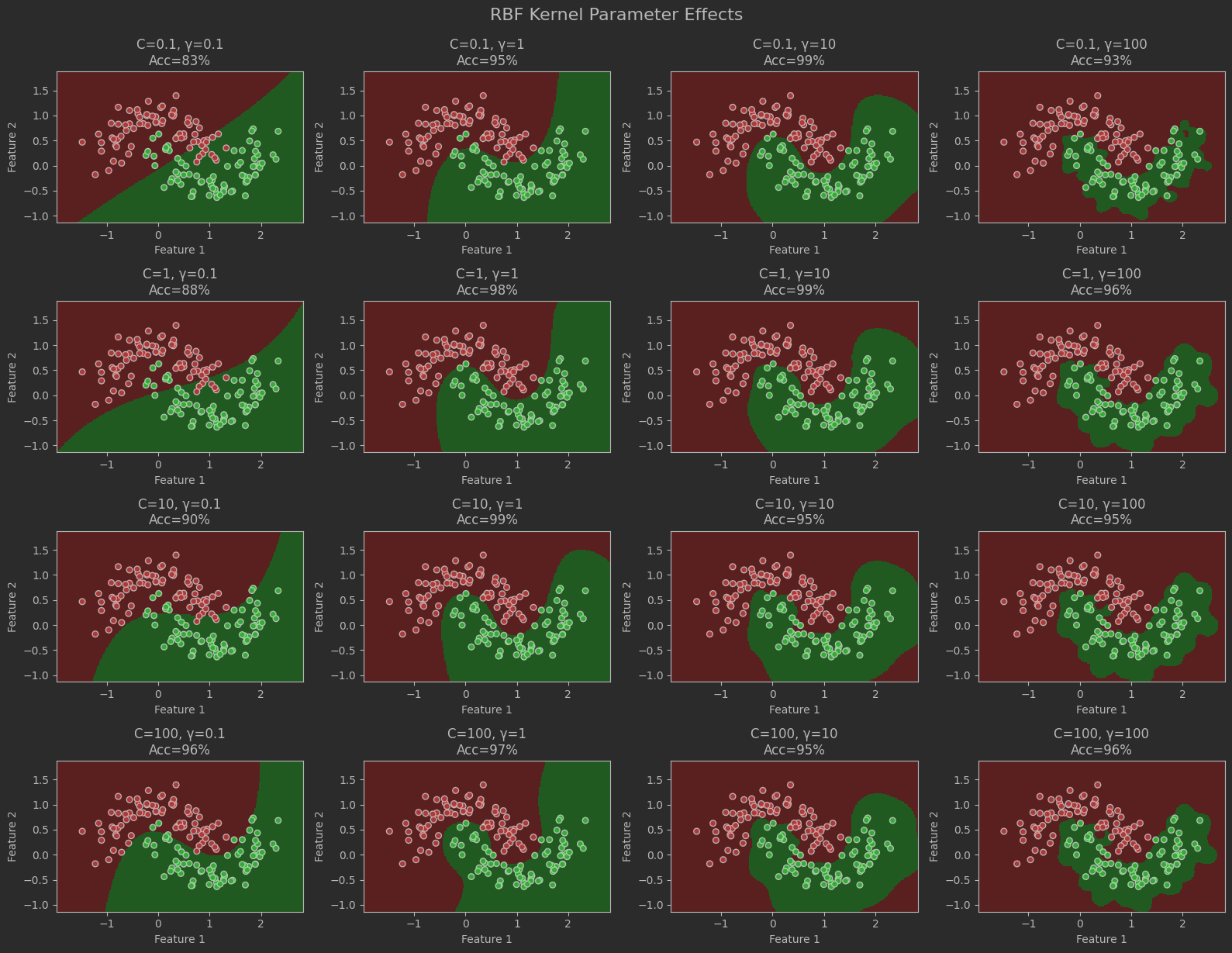

實戰案例：信用卡欺詐檢測的SVM優化分析

案例概述

使用SVM進行信用卡欺詐檢測任務，通過對比不同核函數和參數設置對模型性能的影響，展示在實際場景中如何優化SVM模型。使用Kaggle經典數據集Credit Card Fraud Detection。

數據集特點

??規模??：284,807筆交易（492筆欺詐交易，占比0.172%）
??特征??：28個匿名V變量(V1-V28) + 金額 + 時間
??挑戰??：極度不平衡數據（欺詐僅占0.172%）

代碼實現

import numpy as np
import pandas as pd
import matplotlib.pyplot as plt
import seaborn as sns
from sklearn.model_selection import train_test_split, GridSearchCV
from sklearn.preprocessing import StandardScaler
from sklearn.svm import SVC
from sklearn.metrics import (confusion_matrix, classification_report,precision_recall_curve, PrecisionRecallDisplay,roc_curve, roc_auc_score, f1_score)
from imblearn.over_sampling import SMOTE
from imblearn.pipeline import Pipeline# 設置隨機種子
np.random.seed(42)# 1. 數據加載與準備
df = pd.read_csv('creditcard.csv')# 2. 特征工程
# 創建時間特征
df['hour'] = (df['Time'] % 86400) // 3600# 3. 數據標準化
scaler = StandardScaler()
df[['Amount', 'Time']] = scaler.fit_transform(df[['Amount', 'Time']])# 4. 處理類別不平衡（使用SMOTE）
X = df.drop('Class', axis=1)
y = df['Class']# 5. 數據分割
X_train, X_test, y_train, y_test = train_test_split(X, y, test_size=0.3, stratify=y, random_state=42
)print(f"訓練集形狀: {X_train.shape}, 測試集形狀: {X_test.shape}")
print(f"訓練集欺詐比例: {y_train.mean():.6f}, 測試集欺詐比例: {y_test.mean():.6f}")
#%%
# 創建建模流水線
pipeline = Pipeline([('smote', SMOTE(random_state=42)),  # 處理類別不平衡('clf', SVC(class_weight='balanced', probability=True))  # 設置類別權重
])# 定義參數網格
param_grid = [{'clf__kernel': ['linear'],'clf__C': [0.01, 0.1, 1, 10, 100]},{'clf__kernel': ['rbf'],'clf__C': [0.01, 0.1, 1, 10, 100],'clf__gamma': [0.001, 0.01, 0.1, 1]},{'clf__kernel': ['poly'],'clf__C': [0.01, 0.1, 1, 10],'clf__gamma': [0.001, 0.01, 0.1],'clf__degree': [2, 3]}
]# 執行網格搜索
grid_search = GridSearchCV(pipeline, param_grid,scoring='f1',cv=3,n_jobs=-1,verbose=1
)grid_search.fit(X_train, y_train)# 輸出最佳參數
print("Best parameters:", grid_search.best_params_)
print("Best F1 score:", grid_search.best_score_)# 在測試集上評估最佳模型
best_model = grid_search.best_estimator_
y_pred = best_model.predict(X_test)print("\nClassification Report:")
print(classification_report(y_test, y_pred))print("\nConfusion Matrix:")
print(confusion_matrix(y_test, y_pred))# 保存評估結果
results_df = pd.DataFrame({'Model': [f"{params['clf__kernel']}_C{params['clf__C']}" + (f"_γ{params.get('clf__gamma', '')}" if 'clf__gamma' in params else '') + (f"_d{params.get('clf__degree', '')}" if 'clf__degree' in params else '') for params in grid_search.cv_results_['params']],'F1_Score': grid_search.cv_results_['mean_test_score'],'Parameters': grid_search.cv_results_['params']
})
#%%
plt.figure(figsize=(18, 12))# 1. F1分數比較柱狀圖
plt.subplot(2, 2, 1)
sns.barplot(y='F1_Score',x='Model',data=results_df.sort_values('F1_Score', ascending=False).head(10),palette='viridis'
)
plt.xticks(rotation=45, ha='right')
plt.title('Top 10 SVM Models by F1 Score')
plt.xlabel('Model Configuration')
plt.ylabel('F1 Score')# 2. 混淆矩陣熱力圖
plt.subplot(2, 2, 2)
cm = confusion_matrix(y_test, y_pred)
sns.heatmap(cm, annot=True, fmt='d', cmap='Blues',xticklabels=['Legit', 'Fraud'],yticklabels=['Legit', 'Fraud'])
plt.title('Confusion Matrix - Best Model')
plt.xlabel('Predicted')
plt.ylabel('Actual')# 3. ROC曲線比較
plt.subplot(2, 2, 3)
# 繪制不同模型的ROC曲線
model_combinations = [('Linear (C=0.1)', SVC(kernel='linear', C=0.1, probability=True, class_weight='balanced')),('RBF (C=1, γ=0.1)', SVC(kernel='rbf', C=1, gamma=0.1, probability=True, class_weight='balanced')),('Poly (C=10, γ=0.01, d=3)', SVC(kernel='poly', C=10, gamma=0.01, degree=3, probability=True, class_weight='balanced')),('Best Model', best_model)
]for name, model in model_combinations:model.fit(X_train, y_train)y_proba = model.predict_proba(X_test)[:, 1]fpr, tpr, _ = roc_curve(y_test, y_proba)auc = roc_auc_score(y_test, y_proba)plt.plot(fpr, tpr, label=f'{name} (AUC={auc:.3f})')plt.plot([0, 1], [0, 1], 'k--')
plt.xlabel('False Positive Rate')
plt.ylabel('True Positive Rate')
plt.title('ROC Curve Comparison')
plt.legend(loc='lower right')# 4. 精確率-召回率曲線
plt.subplot(2, 2, 4)
PrecisionRecallDisplay.from_predictions(y_test, best_model.predict_proba(X_test)[:, 1],name=f"Best Model (F1={f1_score(y_test, y_pred):.3f})"
)
plt.title('Precision-Recall Curve')
plt.grid(True)plt.tight_layout()
plt.savefig('svm_comparison.png', dpi=300)
plt.show()