什么是支持向量回歸？ (What is Support Vector Regression?)

Support vector regression is a special kind of regression that gives you some sort of buffer or flexibility with the error. How does it do that ? I’m going to explain it to you in simple terms by showing 2 different graphs.

支持向量回歸是一種特殊的回歸，它為您提供了某種緩沖或靈活的誤差。 它是如何做到的？ 我將通過顯示2個不同的圖形以簡單的方式向您解釋。

The above is an hypothetical linear regression graph. You can see that the regression line is drawn at a position with minimum sqaured errors. Errors are basically the sqaures of difference in distance between the original data point (points in black) and the regression line (predicted values).

上面是一個假設的線性回歸圖。 您可以看到回歸線繪制在具有最小平方誤差的位置。 誤差基本上是原始數據點(黑色的點)與回歸線(預測值)之間的距離差的平方。

The above is the same setting with SVR(Support Vector Regression). You can observe that there are 2 boundaries around the regression line. This is a tube with the vertical distance of epsilon above and below the regression line. In reality, it is kown as epsilon insensitive tube. The role of this tube is that it creates a buffer for the error. To be specific, all the data points within this tube are considered to have zero error from the regression line. Only the points outside of this tube are considered for calculating the errors. The error is calculated as the distance from the data point to the boundary of the tube rather than data point to the regression line (as seen in Linear Regression)

上面與SVR(支持向量回歸)的設置相同。 您可以觀察到回歸線周圍有2個邊界。 這是在回歸線上方和下方都有ε垂直距離的管。 實際上，它被稱為ε敏感管。 該管的作用是為錯誤創建緩沖區。 具體而言，該管內的所有數據點都被認為與回歸線的誤差為零。 僅考慮該管外部的點才能計算誤差。 誤差計算為從數據點到管邊界的距離，而不是從數據點到回歸線的距離(如線性回歸所示)

Why support vector ?

為什么要支持向量？

Well, all the points outside of the tube are known as slack points and they are essentially vectors in a 2-dimensional space. Imagine drawing vectors from the origin to the individual slack points, then you can see all the vectors in the graph. These vectors are supporting the structure or formation of the this tube and hence it is known as support vector regression. You can understand it from the below graph.

好吧，管外的所有點都稱為松弛點，它們本質上是二維空間中的向量。 想象一下從原點到各個松弛點的繪制矢量，然后您可以在圖中看到所有矢量。 這些向量支持該管的結構或形成，因此被稱為支持向量回歸。 您可以從下圖了解它。

用Python實現 (Implementation in Python)

Let us deep dive into python and build a random forest regression model and try to predict the salary of an employee of 6.5 level(hypothetical).

讓我們深入研究python并建立一個隨機森林回歸模型，并嘗試預測6.5級(假設)的員工薪水。

Before you move forward, please download the CSV data file from my GitHub Gist.

在繼續之前，請從我的GitHub Gist下載CSV數據文件。

https://gist.github.com/tharunpeddisetty/3fe7c29e9e56c3e17eb41a376e666083
Once you open the link, you can find "Download Zip" button on the top right corner of the window. Go ahead and download the files.
You can download 1) python file 2)data file (.csv)
Rename the folder accordingly and store it in desired location and you are all set.If you are a beginner I highly recommend you to open your python IDE and follow the steps below because here, I write detailed comments(statements after #.., these do not compile when our run the code) on the working of code. You can use the actual python as your backup file or for your future reference.

Importing Libraries

導入庫

import numpy as np
import matplotlib.pyplot as plt
import pandas as pd

Import Data and Define the X and Y variables

導入數據并定義X和Y變量

dataset = pd.read_csv(‘/Users/tharunpeddisetty/Desktop/Position_Salaries.csv’) #add your file pathX = dataset.iloc[:,1:-1].values
y = dataset.iloc[:, -1].values#iloc takes the values from the specified index locations and stores them in the assigned variable as an array

Let us look at our data and understand the variables:

讓我們看一下數據并了解變量：

This data depicts the position/level of the employee and their salaries. This is the same dataset that I used in my Decision Tree Regression article.

此數據描述了員工的職位/水平及其薪水。 這與我在“決策樹回歸”文章中使用的數據集相同。

Feature Scaling

功能縮放

#Feature Scaling. Required for SVR. Since there’s no concept of coefficients
print(y) 
#we need to reshape y because standard scaler class expects a 2D array
y=y.reshape(len(y),1)from sklearn.preprocessing import StandardScaler
sc_X = StandardScaler()
sc_y = StandardScaler()
X= sc_X.fit_transform(X)
# create a new sc object because the first one calcualtes the mean and standard deviation of X. We need different values of mean and standard deviation for Y
y= sc_y.fit_transform(y)
print(y)

There is no concept of coefficients like linear regression in SVR, so in order to reduce the effect of high valued features we need to scale the features or in other words get all the values under one scale. We achieve this by standardizing the values. Since we have only one feature in this example, we would apply on it anyway. We do that using the StandardScaler() function from sklearn. But, for other datasets, do not forget to scale all your features and the dependent variable. Also, remember to reshape the Y (dependent variable i.e., Salary), which is purely for the sake of passing it through the standard scaler in python.

SVR中沒有像線性回歸這樣的系數概念，因此，為了減少高價值要素的影響，我們需要對要素進行縮放，或者換句話說，將所有值都置于一個尺度下。 我們通過標準化值來實現。 由于在此示例中只有一個功能，因此無論如何我們都可以應用它。 我們使用sklearn的StandardScaler()函數進行此操作。 但是，對于其他數據集，請不要忘記縮放所有特征和因變量。 另外，請記住要重塑Y(因變量，即Salary)，這純粹是為了使其通過python中的標準縮放器。

Training the SVR model

訓練SVR模型

from sklearn.svm import SVR
regressor = SVR(kernel = 'rbf')
regressor.fit(X, y)

Simple, isn’t it ? We are going to use Radial Basis Function as the kernel inside the SVR algorithm. This means that we are using a function called ‘rbf’ in order to map the data from one space to another. Explaining how this works is out of the scope of this article. But, you can always research about it online. The choice of kernel function varies with the distribution of the data. I suggest you research about them after implementing this basic program in python.

很簡單，不是嗎？ 我們將使用徑向基函數作為SVR算法中的內核。 這意味著我們正在使用一個名為“ rbf”的函數，以便將數據從一個空間映射到另一個空間。 解釋其工作原理超出了本文的范圍。 但是，您始終可以在線對其進行研究。 內核功能的選擇隨數據的分布而變化。 我建議您在python中實現此基本程序后，對它們進行研究。

Visualizing the results of SVR Regression

可視化SVR回歸的結果

X_grid = np.arange(min(sc_X.inverse_transform(X)), max(sc_X.inverse_transform(X)), 0.1)
X_grid = X_grid.reshape((len(X_grid), 1))
plt.scatter(sc_X.inverse_transform(X), sc_y.inverse_transform(y), color = 'red')
plt.plot(X_grid, sc_y.inverse_transform(regressor.predict(sc_X.transform(X_grid))), color = 'blue')
plt.title('Support Vector Regression')
plt.xlabel('Position level')
plt.ylabel('Salary')
plt.show()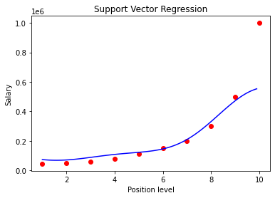

You can see how this model fits to the data. Do you think it is doing a great job ? Compare the results of this with the other regressions that were implemented on the same data in my previous articles and you can see the difference or wait until the end of this article.

您可以看到此模型如何適合數據。 您認為它做得很好嗎？ 將其結果與我以前的文章中基于相同數據實現的其他回歸進行比較，您可以看到差異，或者等到本文結尾。

Predicting 6.5 level result using Decision tree Regression

使用決策樹回歸預測6.5級結果

print(sc_y.inverse_transform(regressor.predict(sc_X.transform([[6.5]])))
)
#We also need to inverse transform in order to get the final result

Make sure you apply all the transformations as that of initial data so that it is easier for the model to recognize the data and produce the relevant results.

確保將所有轉換都應用為原始數據，以便模型更容易識別數據并產生相關結果。

Result

結果

Let me summarize all the results from various regression models so that it is easier for our comparison.

讓我總結各種回歸模型的所有結果，以便我們進行比較。

Support Vector Regression: 170370.0204065

支持向量回歸：170370.0204065

Random Forest Regression: 167000 (Output is not part of the code)

隨機森林回歸：167000(輸出不是代碼的一部分)

Decision Tree Regression: 150000 (Output is not part of the code)

決策樹回歸：150000(輸出不是代碼的一部分)

Polynomial Linear Regression : 158862.45 (Output is not part of the code)

多項式線性回歸：158862.45(輸出不是代碼的一部分)

Linear Regression predicts: 330378.79 (Output is not part of the code)

線性回歸預測：330378.79(輸出不是代碼的一部分)

結論 (Conclusion)

You have the data in front of you. Now, act as a manager and take a decision by yourself. How much salary would you give an employee at 6.5 level (consider level to be the years of experience)? You see, there’s no absolute answer in data science. I can not say that SVR performed better than others, so that is the best model to predict the salaries. If you ask about what I think, I feel the prediction result of random forest regression is realistic than SVR. But again, that is my feeling. Remember that a lot of factors come into play such as position of the employee, average salary in that region for that position and the employee’s previous salary etc. So, don’t even believe me if I say random forest result is the best one. I only said that it is more realistic than others. The end decision depends on the business case of the organization and by no means there is a perfect model to predict the salary of the employee perfectly.

數據就擺在您面前。 現在，擔任經理并自己做出決定。 您會給6.5級的員工多少薪水(考慮到多年的經驗水平)？ 您會發現，數據科學沒有絕對的答案。 我不能說SVR的表現要好于其他，所以這是預測薪資的最佳模型。 如果您問我的想法，我覺得隨機森林回歸的預測結果比SVR更現實。 但是再次，這就是我的感覺。 請記住，許多因素都在起作用，例如員工的職位，該地區在該地區的平均薪水以及員工以前的薪水等。因此，如果我說隨機森林成績是最好的，甚至不要相信我。 我只是說這比其他人更現實。 最終決定取決于組織的業務案例，絕沒有完美的模型可以完美地預測員工的薪水。

Congratulations! You have implemented support vector regression in the minimum lines of code. You now have a template of the code and you can implement this on other datasets and observe results. This marks the end of my articles on regression. Next stop is Classification models. Thanks for reading. Happy Machine Learning!

恭喜你！ 您已在最少的代碼行中實現了支持向量回歸。 現在，您有了代碼模板，您可以在其他數據集上實現此模板并觀察結果。 這標志著我有關回歸的文章的結尾。 下一站是分類模型。 謝謝閱讀。 快樂的機器學習！