文章目錄
- 支持向量機
- 實例1 線性可分的支持向量機
- 1.1 數據讀取
- 1.2 準備訓練數據
- 1.3 實例化線性支持向量機
- 1.4 可視化分析
- 實例2 核支持向量機
- 2.1 讀取數據集
- 2.2 定義高斯核函數
- 2.3 創建非線性的支持向量機
- 2.4 可視化樣本類別
- 實例3 如何選擇最優的C和gamma
- 3.1 讀取數據
- 3.2 利用數據集中的驗證集做模型選擇
- 實例4 基于鳶尾花數據集的決策邊界繪制
- 4.1 讀取鳶尾花數據集(特征選擇花萼長度和花萼寬度)
- 4.2 隨機繪制幾條決策邊界可視化
- 4.3 隨機繪制幾條決策邊界可視化
- 4.4 最大間隔決策邊界可視化
- 實例5 特征是否應該進行標準化?
- 5.1 原始特征的決策邊界可視化
- 5.1 標準化特征的決策邊界可視化
- 實例6
- 實例7 非線性可分的決策邊界
- 7.1 做一個新的數據
- 7.2 繪制高高線表示預測結果
- 7.3 繪制原始數據
- 7.4 繪制不同gamma和C對應的
- 實例8* 手寫SVM
- 8.1 創建數據
- 8.2 定義支持向量機
- 8.3 初始化支持向量機并擬合
- 8.4 支持向量機得到分數
- 實驗1 采用以下數據作為數據集,分別基于線性和核支持向量機進行分類,對于線性核繪制決策邊界
- 1 獲取數據
- 2 可視化數據
- 3 試試采用線性支持向量機來擬合
- 4 試試采用核支持向量機
- 5 繪制線性支持向量機的決策邊界
- 6 繪制非線性決策邊界
支持向量機
在本練習中,我們將使用支持向量機(SVM)來構建垃圾郵件分類器。 我們將從一些簡單的2D數據集開始使用SVM來查看它們的工作原理。 然后,我們將對一組原始電子郵件進行一些預處理工作,并使用SVM在處理的電子郵件上構建分類器,以確定它們是否為垃圾郵件。
我們要做的第一件事是看一個簡單的二維數據集,看看線性SVM如何對數據集進行不同的C值(類似于線性/邏輯回歸中的正則化項)。
實例1 線性可分的支持向量機
1.1 數據讀取
import numpy as np
import pandas as pd
import matplotlib.pyplot as plt
import seaborn as sb
import warnings
warnings.simplefilter("ignore")
我們將其用散點圖表示,其中類標簽由符號表示(+表示正類,o表示負類)。
data1 = pd.read_csv('data/svmdata1.csv')
data1.head()
| X1 | X2 | y | |
|---|---|---|---|
| 0 | 1.9643 | 4.5957 | 1 |
| 1 | 2.2753 | 3.8589 | 1 |
| 2 | 2.9781 | 4.5651 | 1 |
| 3 | 2.9320 | 3.5519 | 1 |
| 4 | 3.5772 | 2.8560 | 1 |
positive=data1[data1["y"].isin([1])]
negative=data1[data1["y"].isin([0])]
negative
| X1 | X2 | y | |
|---|---|---|---|
| 20 | 1.58410 | 3.3575 | 0 |
| 21 | 2.01030 | 3.2039 | 0 |
| 22 | 1.95270 | 2.7843 | 0 |
| 23 | 2.27530 | 2.7127 | 0 |
| 24 | 2.30990 | 2.9584 | 0 |
| 25 | 2.82830 | 2.6309 | 0 |
| 26 | 3.04730 | 2.2931 | 0 |
| 27 | 2.48270 | 2.0373 | 0 |
| 28 | 2.50570 | 2.3853 | 0 |
| 29 | 1.87210 | 2.0577 | 0 |
| 30 | 2.01030 | 2.3546 | 0 |
| 31 | 1.22690 | 2.3239 | 0 |
| 32 | 1.89510 | 2.9174 | 0 |
| 33 | 1.56100 | 3.0709 | 0 |
| 34 | 1.54950 | 2.6923 | 0 |
| 35 | 1.68780 | 2.4057 | 0 |
| 36 | 1.49190 | 2.0271 | 0 |
| 37 | 0.96200 | 2.6820 | 0 |
| 38 | 1.16930 | 2.9276 | 0 |
| 39 | 0.81220 | 2.9992 | 0 |
| 40 | 0.97350 | 3.3881 | 0 |
| 41 | 1.25000 | 3.1937 | 0 |
| 42 | 1.31910 | 3.5109 | 0 |
| 43 | 2.22920 | 2.2010 | 0 |
| 44 | 2.44820 | 2.6411 | 0 |
| 45 | 2.79380 | 1.9656 | 0 |
| 46 | 2.09100 | 1.6177 | 0 |
| 47 | 2.54030 | 2.8867 | 0 |
| 48 | 0.90440 | 3.0198 | 0 |
| 49 | 0.76615 | 2.5899 | 0 |
positive = data1[data1['y'].isin([1])]
negative = data1[data1['y'].isin([0])]
fig, ax = plt.subplots(figsize=(6,4))
ax.scatter(positive['X1'], positive['X2'], s=50, marker='x', label='Positive')
ax.scatter(negative['X1'], negative['X2'], s=50, marker='o', label='Negative')
ax.legend()
plt.show()
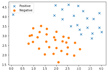
請注意,還有一個異常的正例在其他樣本之外。
這些類仍然是線性分離的,但它非常緊湊。 我們要訓練線性支持向量機來學習類邊界。 在這個練習中,我們沒有從頭開始執行SVM的任務,所以用scikit-learn。
1.2 準備訓練數據
在這里,我們不準備測試數據,直接用所有數據訓練,然后查看訓練完成后,每個點屬于這個類別的置信度
X_train=data1[["X1","X2"]].values
y_train=data1["y"].values
1.3 實例化線性支持向量機
#建立第一個支持向量機對象,C=1
from sklearn import svm
svc1=svm.LinearSVC(C=1,loss="hinge",max_iter=1000)
svc1.fit(X_train,y_train)
svc1.score(X_train,y_train)
0.9803921568627451
from sklearn.model_selection import cross_val_score
cross_val_score(svc1,X_train,y_train,cv=5).mean()
0.9800000000000001
讓我們看看如果C的值越大,會發生什么
#建立第二個支持向量機對象C=100
svc2=svm.LinearSVC(C=100,loss="hinge",max_iter=1000)
svc2.fit(X_train,y_train)
svc2.score(X_train,y_train)
0.9411764705882353
from sklearn.model_selection import cross_val_score
cross_val_score(svc2,X_train,y_train,cv=5).mean()
0.96
X_train.shape
(51, 2)
svc1.decision_function(X_train).shape
(51,)
#建立兩個支持向量機的決策函數
data1["SV1 decision function"]=svc1.decision_function(X_train)
data1["SV2 decision function"]=svc2.decision_function(X_train)
data1
| X1 | X2 | y | SV1 decision function | SV2 decision function | |
|---|---|---|---|---|---|
| 0 | 1.964300 | 4.5957 | 1 | 0.798413 | 4.490754 |
| 1 | 2.275300 | 3.8589 | 1 | 0.380809 | 2.544578 |
| 2 | 2.978100 | 4.5651 | 1 | 1.373025 | 5.668147 |
| 3 | 2.932000 | 3.5519 | 1 | 0.518562 | 2.396315 |
| 4 | 3.577200 | 2.8560 | 1 | 0.332007 | 1.000000 |
| 5 | 4.015000 | 3.1937 | 1 | 0.866642 | 2.621549 |
| 6 | 3.381400 | 3.4291 | 1 | 0.684095 | 2.571736 |
| 7 | 3.911300 | 4.1761 | 1 | 1.607362 | 5.607368 |
| 8 | 2.782200 | 4.0431 | 1 | 0.830991 | 3.766091 |
| 9 | 2.551800 | 4.6162 | 1 | 1.162616 | 5.294331 |
| 10 | 3.369800 | 3.9101 | 1 | 1.069933 | 4.082890 |
| 11 | 3.104800 | 3.0709 | 1 | 0.228063 | 1.087807 |
| 12 | 1.918200 | 4.0534 | 1 | 0.328403 | 2.712621 |
| 13 | 2.263800 | 4.3706 | 1 | 0.791771 | 4.153238 |
| 14 | 2.655500 | 3.5008 | 1 | 0.313312 | 1.886635 |
| 15 | 3.185500 | 4.2888 | 1 | 1.270111 | 5.052445 |
| 16 | 3.657900 | 3.8692 | 1 | 1.206933 | 4.315328 |
| 17 | 3.911300 | 3.4291 | 1 | 0.997496 | 3.237878 |
| 18 | 3.600200 | 3.1221 | 1 | 0.562860 | 1.872985 |
| 19 | 3.035700 | 3.3165 | 1 | 0.387708 | 1.779986 |
| 20 | 1.584100 | 3.3575 | 0 | -0.437342 | 0.085220 |
| 21 | 2.010300 | 3.2039 | 0 | -0.310676 | 0.133779 |
| 22 | 1.952700 | 2.7843 | 0 | -0.687313 | -1.269605 |
| 23 | 2.275300 | 2.7127 | 0 | -0.554972 | -1.091178 |
| 24 | 2.309900 | 2.9584 | 0 | -0.333914 | -0.268319 |
| 25 | 2.828300 | 2.6309 | 0 | -0.294693 | -0.655467 |
| 26 | 3.047300 | 2.2931 | 0 | -0.440957 | -1.451665 |
| 27 | 2.482700 | 2.0373 | 0 | -0.983720 | -2.972828 |
| 28 | 2.505700 | 2.3853 | 0 | -0.686002 | -1.840056 |
| 29 | 1.872100 | 2.0577 | 0 | -1.328194 | -3.675710 |
| 30 | 2.010300 | 2.3546 | 0 | -1.004062 | -2.560208 |
| 31 | 1.226900 | 2.3239 | 0 | -1.492455 | -3.642407 |
| 32 | 1.895100 | 2.9174 | 0 | -0.612714 | -0.919820 |
| 33 | 1.561000 | 3.0709 | 0 | -0.684991 | -0.852917 |
| 34 | 1.549500 | 2.6923 | 0 | -1.000889 | -2.068296 |
| 35 | 1.687800 | 2.4057 | 0 | -1.153080 | -2.803536 |
| 36 | 1.491900 | 2.0271 | 0 | -1.578039 | -4.250726 |
| 37 | 0.962000 | 2.6820 | 0 | -1.356765 | -2.839519 |
| 38 | 1.169300 | 2.9276 | 0 | -1.033648 | -1.799875 |
| 39 | 0.812200 | 2.9992 | 0 | -1.186393 | -2.021672 |
| 40 | 0.973500 | 3.3881 | 0 | -0.773489 | -0.585307 |
| 41 | 1.250000 | 3.1937 | 0 | -0.768670 | -0.854355 |
| 42 | 1.319100 | 3.5109 | 0 | -0.468833 | 0.238673 |
| 43 | 2.229200 | 2.2010 | 0 | -1.000000 | -2.772247 |
| 44 | 2.448200 | 2.6411 | 0 | -0.511169 | -1.100940 |
| 45 | 2.793800 | 1.9656 | 0 | -0.858263 | -2.809175 |
| 46 | 2.091000 | 1.6177 | 0 | -1.557954 | -4.796212 |
| 47 | 2.540300 | 2.8867 | 0 | -0.256185 | -0.206115 |
| 48 | 0.904400 | 3.0198 | 0 | -1.115044 | -1.840424 |
| 49 | 0.766150 | 2.5899 | 0 | -1.547789 | -3.377865 |
| 50 | 0.086405 | 4.1045 | 1 | -0.713261 | 0.571946 |
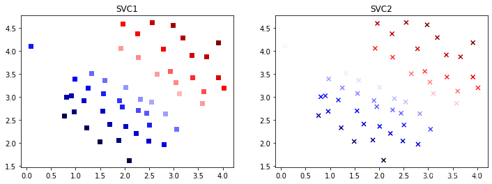
采用決策函數的值作為顏色來看看每個點的置信度,比較兩個支持向量機產生的結果的差異
1.4 可視化分析
#繪制圖片
plt.figure(figsize=(12,4))
plt.subplot(1,2,1)
plt.scatter(data1["X1"],data1["X2"],marker="s",c=data1["SV1 decision function"],cmap='seismic')
plt.title("SVC1")
plt.subplot(1,2,2)
plt.scatter(data1["X1"],data1["X2"],marker="x",c=data1["SV2 decision function"],cmap='seismic')
plt.title("SVC2")
plt.show()
實例2 核支持向量機
現在我們將從線性SVM轉移到能夠使用內核進行非線性分類的SVM。 我們首先負責實現一個高斯核函數。 雖然scikit-learn具有內置的高斯內核,但為了實現更清楚,我們將從頭開始實現。
2.1 讀取數據集
data2 = pd.read_csv('data/svmdata2.csv')
data2
| X1 | X2 | y | |
|---|---|---|---|
| 0 | 0.107143 | 0.603070 | 1 |
| 1 | 0.093318 | 0.649854 | 1 |
| 2 | 0.097926 | 0.705409 | 1 |
| 3 | 0.155530 | 0.784357 | 1 |
| 4 | 0.210829 | 0.866228 | 1 |
| ... | ... | ... | ... |
| 858 | 0.994240 | 0.516667 | 1 |
| 859 | 0.964286 | 0.472807 | 1 |
| 860 | 0.975806 | 0.439474 | 1 |
| 861 | 0.989631 | 0.425439 | 1 |
| 862 | 0.996544 | 0.414912 | 1 |
863 rows × 3 columns
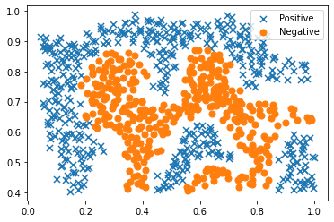
#可視化數據點
positive = data2[data2['y'].isin([1])]
negative = data2[data2['y'].isin([0])]
fig, ax = plt.subplots(figsize=(6,4))
ax.scatter(positive['X1'], positive['X2'], s=50, marker='x', label='Positive')
ax.scatter(negative['X1'], negative['X2'], s=50, marker='o', label='Negative')
ax.legend()
plt.show()
2.2 定義高斯核函數
def gaussian(x1,x2,sigma):return np.exp(-np.sum((x1-x2)**2)/(2*(sigma**2)))
x1=np.arange(1,5)
x2=np.arange(6,10)
gaussian(x1,x2,2)
3.726653172078671e-06
x1 = np.array([1.0, 2.0, 1.0])
x2 = np.array([0.0, 4.0, -1.0])
sigma = 2
gaussian(x1,x2,2)
0.32465246735834974
X2_train=data2[["X1","X2"]].values
y2_train=data2["y"].values
X2_train,y2_train
(array([[0.107143 , 0.60307 ],[0.093318 , 0.649854 ],[0.0979263, 0.705409 ],...,[0.975806 , 0.439474 ],[0.989631 , 0.425439 ],[0.996544 , 0.414912 ]]),array([1, 1, 1, 1, 1, 1, 1, 1, 1, 1, 1, 1, 1, 1, 1, 1, 1, 1, 1, 1, 1, 1,1, 1, 1, 1, 1, 1, 1, 1, 1, 1, 1, 1, 1, 1, 1, 1, 1, 1, 1, 1, 1, 1,1, 1, 1, 1, 1, 1, 1, 1, 1, 1, 1, 1, 1, 1, 1, 1, 1, 1, 1, 1, 1, 1,1, 1, 1, 1, 1, 1, 1, 1, 1, 1, 1, 1, 1, 1, 1, 1, 1, 1, 1, 1, 1, 1,1, 1, 1, 1, 1, 1, 1, 1, 1, 1, 1, 1, 1, 1, 1, 1, 1, 1, 1, 1, 1, 1,1, 1, 1, 1, 1, 1, 1, 1, 1, 1, 1, 1, 1, 1, 1, 1, 1, 1, 1, 1, 1, 1,1, 1, 1, 1, 1, 1, 1, 1, 1, 1, 1, 1, 1, 1, 1, 1, 1, 1, 1, 1, 1, 1,1, 1, 1, 1, 1, 1, 1, 1, 1, 1, 1, 1, 1, 1, 1, 1, 1, 1, 1, 1, 1, 1,1, 1, 1, 1, 1, 1, 1, 1, 1, 1, 1, 1, 1, 1, 1, 1, 1, 0, 0, 0, 0, 0,0, 0, 0, 0, 0, 0, 0, 0, 0, 0, 0, 0, 0, 0, 0, 0, 0, 0, 0, 0, 0, 0,0, 0, 0, 0, 0, 0, 0, 0, 0, 0, 0, 0, 0, 0, 0, 0, 0, 0, 0, 0, 0, 0,0, 0, 0, 0, 0, 0, 0, 0, 0, 0, 0, 0, 0, 0, 0, 0, 0, 0, 0, 0, 0, 0,0, 0, 0, 0, 0, 0, 0, 0, 0, 0, 0, 0, 0, 0, 0, 0, 0, 0, 0, 0, 0, 0,0, 0, 0, 0, 0, 0, 0, 0, 0, 0, 0, 0, 0, 0, 0, 0, 0, 0, 0, 0, 0, 0,0, 0, 0, 0, 0, 0, 0, 0, 0, 0, 0, 0, 0, 0, 0, 0, 1, 1, 1, 1, 1, 1,1, 1, 1, 1, 1, 1, 1, 1, 1, 1, 1, 1, 1, 1, 1, 1, 1, 1, 1, 1, 1, 1,1, 1, 1, 1, 1, 1, 1, 1, 1, 1, 1, 1, 1, 1, 1, 1, 1, 1, 1, 1, 1, 1,1, 1, 1, 0, 0, 0, 0, 0, 0, 0, 0, 0, 0, 0, 0, 0, 0, 0, 0, 0, 0, 0,0, 0, 0, 0, 0, 0, 0, 0, 0, 0, 1, 1, 1, 1, 1, 1, 1, 1, 1, 1, 1, 1,1, 1, 1, 1, 1, 1, 1, 1, 1, 1, 1, 1, 1, 1, 1, 1, 1, 1, 1, 1, 1, 1,1, 1, 1, 1, 1, 1, 1, 1, 1, 1, 1, 1, 1, 0, 0, 0, 0, 0, 0, 0, 0, 0,0, 0, 0, 0, 0, 0, 0, 0, 0, 0, 0, 0, 0, 0, 0, 0, 0, 0, 0, 0, 0, 0,0, 0, 0, 0, 0, 0, 0, 0, 0, 0, 0, 0, 0, 0, 0, 0, 0, 0, 0, 0, 0, 0,0, 0, 0, 0, 0, 0, 0, 0, 0, 0, 0, 1, 1, 1, 1, 1, 1, 1, 1, 1, 1, 1,1, 1, 1, 1, 1, 1, 1, 1, 1, 1, 1, 1, 1, 1, 1, 0, 0, 0, 0, 0, 0, 0,0, 0, 0, 0, 0, 0, 0, 0, 0, 0, 0, 0, 0, 0, 0, 0, 0, 0, 0, 0, 0, 0,0, 0, 0, 0, 1, 1, 1, 1, 1, 1, 1, 1, 1, 1, 1, 1, 1, 1, 1, 1, 1, 1,1, 1, 1, 1, 1, 1, 1, 1, 1, 1, 1, 1, 1, 1, 1, 1, 1, 1, 1, 1, 1, 1,1, 1, 1, 1, 1, 1, 0, 0, 0, 0, 0, 0, 0, 0, 0, 0, 0, 0, 0, 0, 0, 0,0, 0, 0, 0, 0, 0, 0, 0, 0, 0, 0, 0, 0, 0, 0, 0, 0, 0, 0, 0, 0, 0,0, 0, 0, 0, 0, 0, 0, 0, 0, 0, 0, 0, 0, 0, 0, 0, 0, 0, 0, 0, 0, 0,0, 0, 0, 0, 0, 1, 1, 1, 1, 1, 1, 1, 1, 1, 1, 1, 1, 1, 1, 1, 1, 1,1, 1, 1, 1, 1, 1, 1, 1, 1, 1, 1, 1, 1, 1, 1, 1, 1, 1, 1, 1, 1, 1,1, 1, 1, 1, 1, 1, 1, 1, 1, 1, 1, 1, 1, 1, 1, 1, 1, 1, 1, 1, 1, 1,1, 1, 1, 1, 0, 0, 0, 0, 0, 0, 0, 0, 0, 0, 0, 0, 0, 0, 0, 0, 0, 0,0, 0, 0, 0, 0, 0, 0, 0, 0, 0, 0, 0, 0, 0, 0, 0, 0, 0, 0, 0, 0, 0,0, 0, 0, 0, 0, 0, 0, 0, 0, 0, 0, 0, 0, 0, 0, 0, 0, 0, 0, 0, 0, 1,1, 1, 1, 1, 1, 1, 1, 1, 1, 1, 1, 1, 1, 1, 1, 1, 1, 1, 1, 1, 1, 1,1, 1, 1, 1, 1, 1, 1, 1, 1, 1, 1, 1, 1, 1, 1, 1, 1, 1, 1, 1, 1, 1,1, 1, 1, 1, 1], dtype=int64))
該結果與練習中的預期值相符。 接下來,我們將檢查另一個數據集,這次用非線性決策邊界。
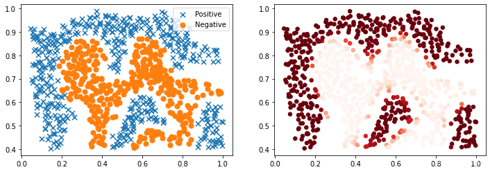
對于該數據集,我們將使用內置的RBF內核構建支持向量機分類器,并檢查其對訓練數據的準確性。 為了可視化決策邊界,這一次我們將根據實例具有負類標簽的預測概率來對點做陰影。 從結果可以看出,它們大部分是正確的。
2.3 創建非線性的支持向量機
import sklearn.svm as svm
nl_svc=svm.SVC(C=100,gamma=10,probability=True)
nl_svc.fit(X2_train,y2_train)
SVC(C=100, gamma=10, probability=True)
nl_svc.score(X2_train,y2_train)
0.9698725376593279
2.4 可視化樣本類別
#將樣本屬于正類的概率作為顏色來對兩類樣本進行可視化輸出
plt.figure(figsize=(12,4))
plt.subplot(1,2,1)
positive = data2[data2['y'].isin([1])]
negative = data2[data2['y'].isin([0])]
plt.scatter(positive['X1'], positive['X2'], s=50, marker='x', label='Positive')
plt.scatter(negative['X1'], negative['X2'], s=50, marker='o', label='Negative')
plt.legend()
plt.subplot(1,2,2)
data2["probability"]=nl_svc.predict_proba(data2[["X1","X2"]])[:,1]
plt.scatter(data2["X1"],data2["X2"],s=30,c=data2["probability"],cmap="Reds")
plt.show()
對于第三個數據集,我們給出了訓練和驗證集,并且基于驗證集性能為SVM模型找到最優超參數。 雖然我們可以使用scikit-learn的內置網格搜索來做到這一點,但是本著遵循練習的目的,我們將從頭開始實現一個簡單的網格搜索。
實例3 如何選擇最優的C和gamma
3.1 讀取數據
#讀取文件,獲取數據集
data3=pd.read_csv('data/svmdata3.csv')
#讀取文件,獲取驗證集
data3val=pd.read_csv('data/svmdata3val.csv')
data3
| X1 | X2 | y | |
|---|---|---|---|
| 0 | -0.158986 | 0.423977 | 1 |
| 1 | -0.347926 | 0.470760 | 1 |
| 2 | -0.504608 | 0.353801 | 1 |
| 3 | -0.596774 | 0.114035 | 1 |
| 4 | -0.518433 | -0.172515 | 1 |
| ... | ... | ... | ... |
| 206 | -0.399885 | -0.621930 | 1 |
| 207 | -0.124078 | -0.126608 | 1 |
| 208 | -0.316935 | -0.228947 | 1 |
| 209 | -0.294124 | -0.134795 | 0 |
| 210 | -0.153111 | 0.184503 | 0 |
211 rows × 3 columns
data3val
| X1 | X2 | yval | y | |
|---|---|---|---|---|
| 0 | -0.353062 | -0.673902 | 0 | 0 |
| 1 | -0.227126 | 0.447320 | 1 | 1 |
| 2 | 0.092898 | -0.753524 | 0 | 0 |
| 3 | 0.148243 | -0.718473 | 0 | 0 |
| 4 | -0.001512 | 0.162928 | 0 | 0 |
| ... | ... | ... | ... | ... |
| 195 | 0.005203 | -0.544449 | 1 | 1 |
| 196 | 0.176352 | -0.572454 | 0 | 0 |
| 197 | 0.127651 | -0.340938 | 0 | 0 |
| 198 | 0.248682 | -0.497502 | 0 | 0 |
| 199 | -0.316899 | -0.429413 | 0 | 0 |
200 rows × 4 columns
X = data3[['X1','X2']].values
Xval = data3val[['X1','X2']].values
y = data3['y'].values
yval = data3val['yval'].values
3.2 利用數據集中的驗證集做模型選擇
C_values = [0.01, 0.03, 0.1, 0.3, 1, 3, 10, 30, 100]
gamma_values = [0.01, 0.03, 0.1, 0.3, 1, 3, 10, 30, 100]best_score = 0
best_params = {'C': None, 'gamma': None}for C in C_values:for gamma in gamma_values:svc = svm.SVC(C=C, gamma=gamma)svc.fit(X, y)score = svc.score(Xval, yval)if score > best_score:best_score = scorebest_params['C'] = Cbest_params['gamma'] = gamma
best_score, best_params
(0.965, {'C': 0.3, 'gamma': 100})
from sklearn import svm, datasets
from sklearn.model_selection import GridSearchCV
parameters = {'gamma':[0.01, 0.03, 0.1, 0.3, 1, 3, 10, 30, 100], 'C': [0.01, 0.03, 0.1, 0.3, 1, 3, 10, 30, 100]}
svc = svm.SVC()
clf = GridSearchCV(svc, parameters)
clf.fit(X, y)
# sorted(clf.cv_results_.keys())
max_index=np.argmax(clf.cv_results_['mean_test_score'])
clf.cv_results_["params"][max_index]
{'C': 30, 'gamma': 3}
實例4 基于鳶尾花數據集的決策邊界繪制
4.1 讀取鳶尾花數據集(特征選擇花萼長度和花萼寬度)
from sklearn.svm import SVC
from sklearn import datasets
import matplotlib as mpl
import matplotlib.pyplot as plt
mpl.rc('axes', labelsize=14)
mpl.rc('xtick', labelsize=12)
mpl.rc('ytick', labelsize=12)
iris = datasets.load_iris()
X = iris["data"][:, (2, 3)]  # petal length, petal width
y = iris["target"]setosa_or_versicolor = (y == 0) | (y == 1)
X = X[setosa_or_versicolor]
y = y[setosa_or_versicolor]# SVM Classifier model
svm_clf = SVC(kernel="linear", C=5)
svm_clf.fit(X, y)
SVC(C=5, kernel='linear')
np.max(X[:,0])
5.1
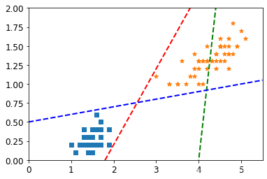
4.2 隨機繪制幾條決策邊界可視化
# Bad models
x0 = np.linspace(0, 5.5, 200)
pred_1 = 5 * x0 - 20
pred_2 = x0 - 1.8
pred_3 = 0.1 * x0 + 0.5
#基于隨機繪制的決策邊界來疊加圖
plt.figure(figsize=(6,4))
plt.plot(x0, pred_1, "g--", linewidth=2)
plt.plot(x0, pred_2, "r--", linewidth=2)
plt.plot(x0, pred_3, "b--", linewidth=2)
plt.scatter(X[:,0][y==0],X[:,1][y==0],marker="s")
plt.scatter(X[:,0][y==1],X[:,1][y==1],marker="*")
plt.axis([0, 5.5, 0, 2])
plt.show()
plt.show()
4.3 隨機繪制幾條決策邊界可視化
svm_clf.coef_[0]
array([1.29411744, 0.82352928])
svm_clf.intercept_[0]
-3.7882347112962464
svm_clf.support_vectors_
array([[1.9, 0.4],[3. , 1.1]])
np.max(X[:,0]),np.min(X[:,0])
(5.1, 1.0)
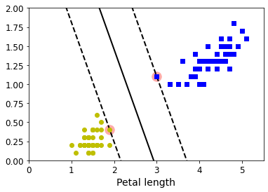
4.4 最大間隔決策邊界可視化
def plot_svc_decision_boundary(svm_clf, xmin, xmax):w = svm_clf.coef_[0]b = svm_clf.intercept_[0]# At the decision boundary, w0*x0 + w1*x1 + b = 0# => x1 = -w0/w1 * x0 - b/w1x0 = np.linspace(xmin, xmax, 200)decision_boundary = -w[0]/w[1] * x0 - b/w[1]# margin = 1/np.sqrt(w[1]**2+w[0]**2)margin = 1/0.9margin = 1/w[1]gutter_up = decision_boundary + margingutter_down = decision_boundary - marginsvs = svm_clf.support_vectors_plt.scatter(svs[:, 0], svs[:, 1], s=180, facecolors='#FFAAAA')plt.plot(x0, decision_boundary, "k-", linewidth=2)plt.plot(x0, gutter_up, "k--", linewidth=2)plt.plot(x0, gutter_down, "k--", linewidth=2)
plt.figure(figsize=(6,4))
plot_svc_decision_boundary(svm_clf, 0, 5.5)
plt.plot(X[:, 0][y == 1], X[:, 1][y == 1], "bs")
plt.plot(X[:, 0][y == 0], X[:, 1][y == 0], "yo")
plt.xlabel("Petal length", fontsize=14)
plt.axis([0, 5.5, 0, 2])plt.show()
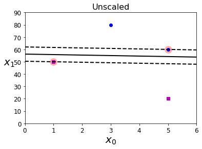
實例5 特征是否應該進行標準化?
5.1 原始特征的決策邊界可視化
#準備數據
Xs = np.array([[1, 50], [5, 20], [3, 80], [5, 60]]).astype(np.float64)
ys = np.array([0, 0, 1, 1])
#實例化模型
svm_clf = SVC(kernel="linear", C=100)
svm_clf.fit(Xs, ys)
#繪制圖形
plt.figure(figsize=(6,4))
plt.plot(Xs[:, 0][ys == 1], Xs[:, 1][ys == 1], "bo")
plt.plot(Xs[:, 0][ys == 0], Xs[:, 1][ys == 0], "ms")
plot_svc_decision_boundary(svm_clf, 0, 6)
plt.xlabel("$x_0$", fontsize=20)
plt.ylabel("$x_1$  ", fontsize=20, rotation=0)
plt.title("Unscaled", fontsize=16)
plt.axis([0, 6, 0, 90])
(0.0, 6.0, 0.0, 90.0)
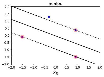
5.1 標準化特征的決策邊界可視化
from sklearn.preprocessing import StandardScaler
scaler = StandardScaler()
X_scaled = scaler.fit_transform(Xs)
svm_clf.fit(X_scaled, ys)
plt.plot(X_scaled[:, 0][ys == 1], X_scaled[:, 1][ys == 1], "bo")
plt.plot(X_scaled[:, 0][ys == 0], X_scaled[:, 1][ys == 0], "ms")
plot_svc_decision_boundary(svm_clf, -2, 2)
plt.xlabel("$x_0$", fontsize=20)
plt.title("Scaled", fontsize=16)
plt.axis([-2, 2, -2, 2])
plt.show()
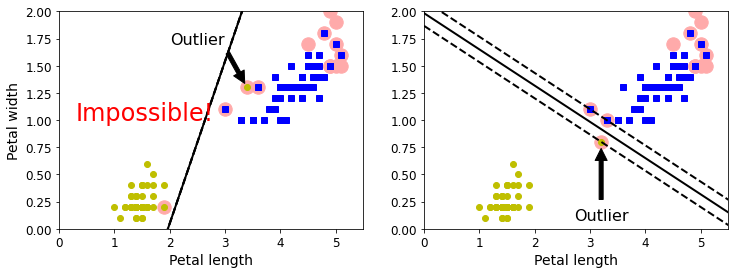
實例6
#回到鳶尾花數據集
X = iris["data"][:, (2, 3)]  # petal length, petal width
y = iris["target"]
X_outliers = np.array([[3.4, 1.3], [3.2, 0.8]])
y_outliers = np.array([0, 0])Xo1 = np.concatenate([X, X_outliers[:1]], axis=0)
yo1 = np.concatenate([y, y_outliers[:1]], axis=0)
Xo2 = np.concatenate([X, X_outliers[1:]], axis=0)
yo2 = np.concatenate([y, y_outliers[1:]], axis=0)svm_clf1= SVC(kernel="linear", C=10**9)
svm_clf1.fit(Xo1, yo1)plt.figure(figsize=(12, 4))plt.subplot(121)
plt.plot(Xo1[:, 0][yo1 == 1], Xo1[:, 1][yo1 == 1], "bs")
plt.plot(Xo1[:, 0][yo1 == 0], Xo1[:, 1][yo1 == 0], "yo")
plt.text(0.3, 1.0, "Impossible!", fontsize=24, color="red")
plot_svc_decision_boundary(svm_clf1, 0, 5.5)
plt.xlabel("Petal length", fontsize=14)
plt.ylabel("Petal width", fontsize=14)
plt.annotate("Outlier",xy=(X_outliers[0][0], X_outliers[0][1]),xytext=(2.5, 1.7),ha="center",arrowprops=dict(facecolor='black', shrink=0.1),fontsize=16,
)
plt.axis([0, 5.5, 0, 2])svm_clf2 = SVC(kernel="linear", C=10**9)
svm_clf2.fit(Xo2, yo2)plt.subplot(122)
plt.plot(Xo2[:, 0][yo2 == 1], Xo2[:, 1][yo2 == 1], "bs")
plt.plot(Xo2[:, 0][yo2 == 0], Xo2[:, 1][yo2 == 0], "yo")
plot_svc_decision_boundary(svm_clf2, 0, 5.5)
plt.xlabel("Petal length", fontsize=14)
plt.annotate("Outlier",xy=(X_outliers[1][0], X_outliers[1][1]),xytext=(3.2, 0.08),ha="center",arrowprops=dict(facecolor='black', shrink=0.1),fontsize=16,
)
plt.axis([0, 5.5, 0, 2])plt.show()
plt.show()
實例7 非線性可分的決策邊界
7.1 做一個新的數據
from sklearn.pipeline import Pipeline
from sklearn.datasets import make_moons
X, y = make_moons(n_samples=100, noise=0.15, random_state=42)
np.min(X[:,0]),np.max(X[:,0])
(-1.2720155884887554, 2.4093807207967215)
np.min(X[:,1]),np.max(X[:,1])
(-0.6491427462708279, 1.2711135917248466)
x0s = np.linspace(2, 15, 2)
x1s = np.linspace(3,12,2)
x0, x1 = np.meshgrid(x0s, x1s)
x0s ,x1s ,x0, x1
(array([ 2., 15.]),array([ 3., 12.]),array([[ 2., 15.],[ 2., 15.]]),array([[ 3., 3.],[12., 12.]]))
x1.ravel()
array([ 3., 3., 12., 12.])
x0.ravel()
array([ 2., 15., 2., 15.])
X = np.c_[x0.ravel(), x1.ravel()]
X.shape,X
((4, 2),array([[ 2., 3.],[15., 3.],[ 2., 12.],[15., 12.]]))
y_pred=np.array([[1,0],[0,1]])
np.meshgrid(x0s, x1s)
[array([[ 2., 15.],[ 2., 15.]]),array([[ 3., 3.],[12., 12.]])]
X = np.c_[x0.ravel(), x1.ravel()]
X.shape,x0.shape
((4, 2), (2, 2))
x0
array([[ 2., 15.],[ 2., 15.]])
7.2 繪制高高線表示預測結果
def plot_predictions(clf, axes):x0s = np.linspace(axes[0], axes[1], 100)x1s = np.linspace(axes[2], axes[3], 100)x0, x1 = np.meshgrid(x0s, x1s)X = np.c_[x0.ravel(), x1.ravel()]y_pred = clf.predict(X).reshape(x0.shape)y_decision = clf.decision_function(X).reshape(x0.shape)plt.contourf(x0, x1, y_pred, cmap=plt.cm.brg, alpha=0.2)plt.contourf(x0, x1, y_decision, cmap=plt.cm.brg, alpha=0.1)
7.3 繪制原始數據
def plot_dataset(X, y, axes):plt.plot(X[:, 0][y==0], X[:, 1][y==0], "bs")plt.plot(X[:, 0][y==1], X[:, 1][y==1], "g^")plt.axis(axes)plt.grid(True, which='both')plt.xlabel(r"$x_1$", fontsize=20)plt.ylabel(r"$x_2$", fontsize=20, rotation=0)
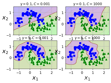
7.4 繪制不同gamma和C對應的
from sklearn.svm import SVCX, y = make_moons(n_samples=100, noise=0.15, random_state=42)
gamma1, gamma2 = 0.1, 5
C1, C2 = 0.001, 1000
hyperparams = (gamma1, C1), (gamma1, C2), (gamma2, C1), (gamma2, C2)svm_clfs = []
for gamma, C in hyperparams:rbf_kernel_svm_clf = Pipeline([("scaler", StandardScaler()),("svm_clf",SVC(kernel="rbf", gamma=gamma, C=C))])rbf_kernel_svm_clf.fit(X, y)svm_clfs.append(rbf_kernel_svm_clf)plt.figure(figsize=(6,4))for i, svm_clf in enumerate(svm_clfs):plt.subplot(221 + i)plot_predictions(svm_clf, [-1.5, 2.5, -1, 1.5])plot_dataset(X, y, [-1.5, 2.5, -1, 1.5])gamma, C = hyperparams[i]plt.title(r"$\gamma = {}, C = {}$".format(gamma, C), fontsize=12)plt.show()
實例8* 手寫SVM
8.1 創建數據
import numpy as np
import pandas as pd
from sklearn.datasets import load_iris
from sklearn.model_selection import  train_test_split
import matplotlib.pyplot as plt
%matplotlib inline
# data
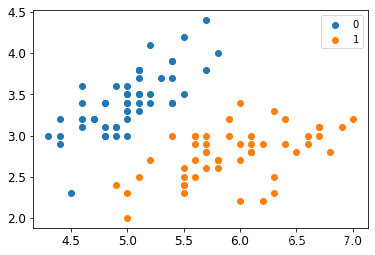
def create_data():iris = load_iris()df = pd.DataFrame(iris.data, columns=iris.feature_names)df['label'] = iris.targetdf.columns = ['sepal length', 'sepal width', 'petal length', 'petal width', 'label']data = np.array(df.iloc[:100, [0, 1, -1]])for i in range(len(data)):if data[i,-1] == 0:data[i,-1] = -1return data[:,:2], data[:,-1]
X, y = create_data()
X_train, X_test, y_train, y_test = train_test_split(X, y, test_size=0.25)
plt.scatter(X[:50,0],X[:50,1], label='0')
plt.scatter(X[50:,0],X[50:,1], label='1')
plt.legend()
<matplotlib.legend.Legend at 0x1c516838670>
8.2 定義支持向量機
class SVM:def __init__(self, max_iter=100, kernel='linear'):self.max_iter = max_iterself._kernel = kerneldef init_args(self, features, labels):self.m, self.n = features.shapeself.X = featuresself.Y = labelsself.b = 0.0# 將Ei保存在一個列表里self.alpha = np.ones(self.m)self.E = [self._E(i) for i in range(self.m)]# 松弛變量self.C = 1.0def _KKT(self, i):y_g = self._g(i) * self.Y[i]if self.alpha[i] == 0:return y_g >= 1elif 0 < self.alpha[i] < self.C:return y_g == 1else:return y_g <= 1# g(x)預測值,輸入xi(X[i])def _g(self, i):r = self.bfor j in range(self.m):r += self.alpha[j] * self.Y[j] * self.kernel(self.X[i], self.X[j])return r# 核函數def kernel(self, x1, x2):if self._kernel == 'linear':return sum([x1[k] * x2[k] for k in range(self.n)])elif self._kernel == 'poly':return (sum([x1[k] * x2[k] for k in range(self.n)]) + 1)**2return 0# E(x)為g(x)對輸入x的預測值和y的差def _E(self, i):return self._g(i) - self.Y[i]def _init_alpha(self):# 外層循環首先遍歷所有滿足0<a<C的樣本點,檢驗是否滿足KKTindex_list = [i for i in range(self.m) if 0 < self.alpha[i] < self.C]# 否則遍歷整個訓練集non_satisfy_list = [i for i in range(self.m) if i not in index_list]index_list.extend(non_satisfy_list)for i in index_list:if self._KKT(i):continueE1 = self.E[i]# 如果E2是+,選擇最小的;如果E2是負的,選擇最大的if E1 >= 0:j = min(range(self.m), key=lambda x: self.E[x])else:j = max(range(self.m), key=lambda x: self.E[x])return i, jdef _compare(self, _alpha, L, H):if _alpha > H:return Helif _alpha < L:return Lelse:return _alphadef fit(self, features, labels):self.init_args(features, labels)for t in range(self.max_iter):# traini1, i2 = self._init_alpha()# 邊界if self.Y[i1] == self.Y[i2]:L = max(0, self.alpha[i1] + self.alpha[i2] - self.C)H = min(self.C, self.alpha[i1] + self.alpha[i2])else:L = max(0, self.alpha[i2] - self.alpha[i1])H = min(self.C, self.C + self.alpha[i2] - self.alpha[i1])E1 = self.E[i1]E2 = self.E[i2]# eta=K11+K22-2K12eta = self.kernel(self.X[i1], self.X[i1]) + self.kernel(self.X[i2],self.X[i2]) - 2 * self.kernel(self.X[i1], self.X[i2])if eta <= 0:# print('eta <= 0')continuealpha2_new_unc = self.alpha[i2] + self.Y[i2] * (E1 - E2) / eta #此處有修改,根據書上應該是E1 - E2,書上130-131頁alpha2_new = self._compare(alpha2_new_unc, L, H)alpha1_new = self.alpha[i1] + self.Y[i1] * self.Y[i2] * (self.alpha[i2] - alpha2_new)b1_new = -E1 - self.Y[i1] * self.kernel(self.X[i1], self.X[i1]) * (alpha1_new - self.alpha[i1]) - self.Y[i2] * self.kernel(self.X[i2],self.X[i1]) * (alpha2_new - self.alpha[i2]) + self.bb2_new = -E2 - self.Y[i1] * self.kernel(self.X[i1], self.X[i2]) * (alpha1_new - self.alpha[i1]) - self.Y[i2] * self.kernel(self.X[i2],self.X[i2]) * (alpha2_new - self.alpha[i2]) + self.bif 0 < alpha1_new < self.C:b_new = b1_newelif 0 < alpha2_new < self.C:b_new = b2_newelse:# 選擇中點b_new = (b1_new + b2_new) / 2# 更新參數self.alpha[i1] = alpha1_newself.alpha[i2] = alpha2_newself.b = b_newself.E[i1] = self._E(i1)self.E[i2] = self._E(i2)return 'train done!'def predict(self, data):r = self.bfor i in range(self.m):r += self.alpha[i] * self.Y[i] * self.kernel(data, self.X[i])return 1 if r > 0 else -1def score(self, X_test, y_test):right_count = 0for i in range(len(X_test)):result = self.predict(X_test[i])if result == y_test[i]:right_count += 1return right_count / len(X_test)def _weight(self):# linear modelyx = self.Y.reshape(-1, 1) * self.Xself.w = np.dot(yx.T, self.alpha)return self.w
8.3 初始化支持向量機并擬合
svm = SVM(max_iter=100)
svm.fit(X_train, y_train)
'train done!'
8.4 支持向量機得到分數
svm.score(X_test, y_test)
0.72
實驗1 采用以下數據作為數據集,分別基于線性和核支持向量機進行分類,對于線性核繪制決策邊界
1 獲取數據
from sklearn.svm import SVC
from sklearn import datasets
import matplotlib as mpl
import matplotlib.pyplot as plt
mpl.rc('axes', labelsize=14)
mpl.rc('xtick', labelsize=12)
mpl.rc('ytick', labelsize=12)
iris = datasets.load_iris()
X = iris["data"][:, (2, 3)]  # petal length, petal width
y = iris["target"]
X,y
(array([[1.4, 0.2],[1.4, 0.2],[1.3, 0.2],[1.5, 0.2],[1.4, 0.2],[1.7, 0.4],[1.4, 0.3],[1.5, 0.2],[1.4, 0.2],[1.5, 0.1],[1.5, 0.2],[1.6, 0.2],[1.4, 0.1],[1.1, 0.1],[1.2, 0.2],[1.5, 0.4],[1.3, 0.4],[1.4, 0.3],[1.7, 0.3],[1.5, 0.3],[1.7, 0.2],[1.5, 0.4],[1. , 0.2],[1.7, 0.5],[1.9, 0.2],[1.6, 0.2],[1.6, 0.4],[1.5, 0.2],[1.4, 0.2],[1.6, 0.2],[1.6, 0.2],[1.5, 0.4],[1.5, 0.1],[1.4, 0.2],[1.5, 0.2],[1.2, 0.2],[1.3, 0.2],[1.4, 0.1],[1.3, 0.2],[1.5, 0.2],[1.3, 0.3],[1.3, 0.3],[1.3, 0.2],[1.6, 0.6],[1.9, 0.4],[1.4, 0.3],[1.6, 0.2],[1.4, 0.2],[1.5, 0.2],[1.4, 0.2],[4.7, 1.4],[4.5, 1.5],[4.9, 1.5],[4. , 1.3],[4.6, 1.5],[4.5, 1.3],[4.7, 1.6],[3.3, 1. ],[4.6, 1.3],[3.9, 1.4],[3.5, 1. ],[4.2, 1.5],[4. , 1. ],[4.7, 1.4],[3.6, 1.3],[4.4, 1.4],[4.5, 1.5],[4.1, 1. ],[4.5, 1.5],[3.9, 1.1],[4.8, 1.8],[4. , 1.3],[4.9, 1.5],[4.7, 1.2],[4.3, 1.3],[4.4, 1.4],[4.8, 1.4],[5. , 1.7],[4.5, 1.5],[3.5, 1. ],[3.8, 1.1],[3.7, 1. ],[3.9, 1.2],[5.1, 1.6],[4.5, 1.5],[4.5, 1.6],[4.7, 1.5],[4.4, 1.3],[4.1, 1.3],[4. , 1.3],[4.4, 1.2],[4.6, 1.4],[4. , 1.2],[3.3, 1. ],[4.2, 1.3],[4.2, 1.2],[4.2, 1.3],[4.3, 1.3],[3. , 1.1],[4.1, 1.3],[6. , 2.5],[5.1, 1.9],[5.9, 2.1],[5.6, 1.8],[5.8, 2.2],[6.6, 2.1],[4.5, 1.7],[6.3, 1.8],[5.8, 1.8],[6.1, 2.5],[5.1, 2. ],[5.3, 1.9],[5.5, 2.1],[5. , 2. ],[5.1, 2.4],[5.3, 2.3],[5.5, 1.8],[6.7, 2.2],[6.9, 2.3],[5. , 1.5],[5.7, 2.3],[4.9, 2. ],[6.7, 2. ],[4.9, 1.8],[5.7, 2.1],[6. , 1.8],[4.8, 1.8],[4.9, 1.8],[5.6, 2.1],[5.8, 1.6],[6.1, 1.9],[6.4, 2. ],[5.6, 2.2],[5.1, 1.5],[5.6, 1.4],[6.1, 2.3],[5.6, 2.4],[5.5, 1.8],[4.8, 1.8],[5.4, 2.1],[5.6, 2.4],[5.1, 2.3],[5.1, 1.9],[5.9, 2.3],[5.7, 2.5],[5.2, 2.3],[5. , 1.9],[5.2, 2. ],[5.4, 2.3],[5.1, 1.8]]),array([0, 0, 0, 0, 0, 0, 0, 0, 0, 0, 0, 0, 0, 0, 0, 0, 0, 0, 0, 0, 0, 0,0, 0, 0, 0, 0, 0, 0, 0, 0, 0, 0, 0, 0, 0, 0, 0, 0, 0, 0, 0, 0, 0,0, 0, 0, 0, 0, 0, 1, 1, 1, 1, 1, 1, 1, 1, 1, 1, 1, 1, 1, 1, 1, 1,1, 1, 1, 1, 1, 1, 1, 1, 1, 1, 1, 1, 1, 1, 1, 1, 1, 1, 1, 1, 1, 1,1, 1, 1, 1, 1, 1, 1, 1, 1, 1, 1, 1, 2, 2, 2, 2, 2, 2, 2, 2, 2, 2,2, 2, 2, 2, 2, 2, 2, 2, 2, 2, 2, 2, 2, 2, 2, 2, 2, 2, 2, 2, 2, 2,2, 2, 2, 2, 2, 2, 2, 2, 2, 2, 2, 2, 2, 2, 2, 2, 2, 2]))
X_train=X[(y==1) | (y==2)]
y_train=y[(y==1) | (y==2)]
y_train
array([1, 1, 1, 1, 1, 1, 1, 1, 1, 1, 1, 1, 1, 1, 1, 1, 1, 1, 1, 1, 1, 1,1, 1, 1, 1, 1, 1, 1, 1, 1, 1, 1, 1, 1, 1, 1, 1, 1, 1, 1, 1, 1, 1,1, 1, 1, 1, 1, 1, 2, 2, 2, 2, 2, 2, 2, 2, 2, 2, 2, 2, 2, 2, 2, 2,2, 2, 2, 2, 2, 2, 2, 2, 2, 2, 2, 2, 2, 2, 2, 2, 2, 2, 2, 2, 2, 2,2, 2, 2, 2, 2, 2, 2, 2, 2, 2, 2, 2])
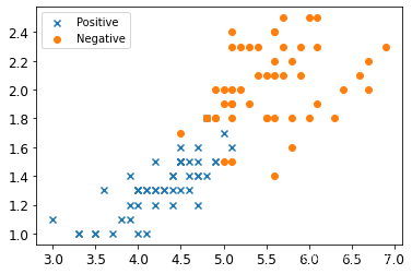
2 可視化數據
plt.scatter(X_train[:50,0],X_train[:50,1],marker='x',label='Positive')
plt.scatter(X_train[50:,0],X_train[50:,1],marker='o',label='Negative')
plt.legend()
<matplotlib.legend.Legend at 0x1c515115610>
3 試試采用線性支持向量機來擬合
from sklearn.svm import SVC
svm_clf = SVC(kernel="linear", C=10,max_iter=1000)
svm_clf.fit(X_train,y_train)
SVC(C=10, kernel='linear', max_iter=1000)
svm_clf.score(X_train,y_train)
0.95
4 試試采用核支持向量機
import sklearn.svm as svm
nl_svc=svm.SVC(C=1,gamma=1,probability=True)
nl_svc.fit(X_train,y_train)
nl_svc.score(X_train,y_train)
0.95
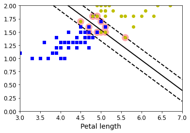
5 繪制線性支持向量機的決策邊界
def plot_svc_decision_boundary(svm_clf, xmin, xmax):w = svm_clf.coef_[0]b = svm_clf.intercept_[0]# At the decision boundary, w0*x0 + w1*x1 + b = 0# => x1 = -w0/w1 * x0 - b/w1x0 = np.linspace(xmin, xmax, 200)decision_boundary = -w[0]/w[1] * x0 - b/w[1]# margin = 1/np.sqrt(w[1]**2+w[0]**2)margin = 1/0.9margin = 1/w[1]gutter_up = decision_boundary + margingutter_down = decision_boundary - marginsvs = svm_clf.support_vectors_plt.scatter(svs[:, 0], svs[:, 1], s=180, facecolors='#FFAAAA')plt.plot(x0, decision_boundary, "k-", linewidth=2)plt.plot(x0, gutter_up, "k--", linewidth=2)plt.plot(x0, gutter_down, "k--", linewidth=2)
np.min(X_train[:,0]),np.max(X_train[:,0])
(3.0, 6.9)
plt.figure(figsize=(6,4))
plot_svc_decision_boundary(svm_clf,3,7)
plt.plot(X[:, 0][y == 1], X[:, 1][y == 1], "bs")
plt.plot(X[:, 0][y == 2], X[:, 1][y == 2], "yo")
plt.xlabel("Petal length", fontsize=14)
plt.axis([3,7,0,2])
plt.show()
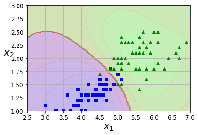
6 繪制非線性決策邊界
def plot_predictions(clf, axes):x0s = np.linspace(axes[0], axes[1], 100)x1s = np.linspace(axes[2], axes[3], 100)x0, x1 = np.meshgrid(x0s, x1s)X = np.c_[x0.ravel(), x1.ravel()]y_pred = clf.predict(X).reshape(x0.shape)y_decision = clf.decision_function(X).reshape(x0.shape)plt.contourf(x0, x1, y_pred, cmap=plt.cm.brg, alpha=0.2)plt.contourf(x0, x1, y_decision, cmap=plt.cm.brg, alpha=0.1)
def plot_dataset(X, y, axes):plt.plot(X[:, 0][y==1], X[:, 1][y==1], "bs")plt.plot(X[:, 0][y==2], X[:, 1][y==2], "g^")plt.axis(axes)plt.grid(True, which='both')plt.xlabel(r"$x_1$", fontsize=20)plt.ylabel(r"$x_2$", fontsize=20, rotation=0)
np.min(X_train[:,0]),np.max(X_train[:,0]),
(3.0, 6.9)
np.min(X_train[:,1]),np.max(X_train[:,1])
(1.0, 2.5)
plot_predictions(nl_svc, [2.5,7,1,3])
plot_dataset(X, y, [2.5,7,1,3])
)
)


)
)


 CUDA 硬件實現)


