介紹 (Introduction)

Performing multiple regression analysis from a large set of independent variables can be a challenging task. Identifying the best subset of regressors for a model involves optimizing against things like bias, multicollinearity, exogeneity/endogeneity, and threats to external validity. Such problems become difficult to understand and control in the presence of a large number of features. Professors will often tell you to “let theory be your guide” when going about feature selection, but that is not always so easy.

從大量獨立變量中進行多元回歸分析可能是一項艱巨的任務。 為模型確定最佳的回歸子集涉及針對偏差，多重共線性，外生性/內生性以及對外部有效性的威脅等方面的優化。 在存在大量特征的情況下，此類問題變得難以理解和控制。 在進行特征選擇時，教授通常會告訴您“讓理論作為指導”，但這并不總是那么容易。

This blog considers the issue of multicollinearity and suggests a method of avoiding it. Proposed here is not a “solution” to collinear variables, nor is it a perfect way of identifying them. It is simply one measurement to take into consideration when comparing multiple subsets of variables.

該博客考慮了多重共線性問題，并提出了避免這種問題的方法。 這里提出的不是共線變量的“解決方案”，也不是識別它們的理想方法。 比較變量的多個子集時，它只是一種要考慮的度量。

問題 (The Problem)

There are several ways of identifying the features that are causing problems in a model. The most common approach (and the basis of this post) is to calculate correlations between suspected collinear variables. While effective, it is important to acknowledge the shortcomings of this method. For instance, correlation coefficients are often biased by sample sizes, and bivariate correlation cannot detect two variables that are collinear only in the presence of additional variables. For these reasons, it is a good idea to consider other metrics/methods as well, some of which include the following: look at the significance of coefficients compared to the overall model; look for high standard error; calculate variance inflation factors for different features; conduct principal components analysis; and yes, let theory be your guide.

有幾種方法可以識別導致模型出現問題的特征。 最常見的方法(也是本文的基礎)是計算可疑共線變量之間的相關性。 盡管有效，但重要的是要認識到此方法的缺點。 例如，相關系數通常受樣本量的影響，而雙變量相關僅在存在其他變量的情況下無法檢測到共線的兩個變量。 由于這些原因，考慮其他指標/方法也是一個好主意，其中的一些指標/方法包括：與整體模型相比，考察系數的重要性； 尋找高標準誤差； 計算不同特征的方差膨脹因子； 進行主成分分析； 是的，以理論為指導。

With all of this in mind, let us now consider a technique that employs a collection of transformed Pearson correlation coefficients in a multiple-criteria evaluation problem (see Multiple-Criteria Decision Analysis). The goal of the technique is to find a subset of independent variables where every pairwise correlation within the set is as low as possible, while simultaneously, each variable’s correlation with the dependent variable is as high as possible. We may represent the problem in the following way:

考慮到所有這些，現在讓我們考慮一種在多準則評估問題中使用一組變換的Pearson相關系數的技術(請參閱多準則決策分析 )。 該技術的目標是找到獨立變量的子集，其中集合中每個成對的相關性都應盡可能低，而同時，每個變量與因變量的相關性應盡可能地高。 我們可以通過以下方式表示問題：

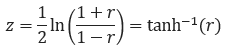
Here, r is the Pearson correlation coefficient of two variables, and f(x) is the weighted mean of a set of correlation coefficients. In order to apply this function, the coefficients must first be transformed in order to correct for their bias. Arithmetic operations are invalid on raw correlation coefficients because unstable variances across different values make them biased estimates of the population. To address this, we apply the Fisher z-transformation, normalizing the distribution of correlations and approximating stable variance. The Fisher z-transformation is denoted as:

在此， r是兩個變量的皮爾遜相關系數， f (x)是一組相關系數的加權平均值。 為了應用該功能，必須首先對系數進行變換以校正其偏差。 算術運算對原始相關系數無效，因為不同值之間的不穩定方差使其成為總體的有偏估計。 為了解決這個問題，我們應用了Fisher z變換，對相關分布進行了歸一化并近似了穩定方差。 Fisher z變換表示為：

With this in mind, we now consider the “maximizing” and “minimizing” elements of the problem. Because the magnitude and not the direction of correlation is of concern, the absolute value of coefficients are considered. We might think of maximizing correlation to mean “get as close to 1 as possible” and minimizing correlation to mean “get as close to 0 as possible”. Getting as close to 1 as possible is less intuitive after applying the z-transformation, because arctanh(1)=∞. Therefore, we can change the maximization problem to a minimization problem by subtracting the absolute value of each correlation from 1. Now, we might phrase the problem as follows:

考慮到這一點，我們現在考慮問題的“最大化”和“最小化”要素。 因為關注的是幅度而不是相關方向，所以考慮了系數的絕對值。 我們可能會想到最大化相關性以表示“盡可能接近1”，最小化相關性以表示“盡可能接近0”。 在應用z變換后，盡可能接近1不太直觀，因為arctanh (1)=∞。 因此，我們可以通過從1中減去每個相關的絕對值，將最大化問題變為最小化問題。現在，我們可以用以下方式表達問題：

We find the set of features that minimizes both of these functions by calculating the distance of each set from the theoretical global minimum (0,0). This solution can be best represented graphically. The figure below plots the two functions against each other for every set of features in a sample dataset. Each blue point represents one subset of variables, while the red area is an arbitrary frontier to visualize which point has the shortest Euclidian distance from the theoretical minimum.

通過計算每個集合與理論全局最小值(0,0)的距離，我們找到了使這兩個函數最小化的特征集。 該解決方案最好以圖形方式表示。 下圖針對樣本數據集中的每組特征繪制了兩個函數的相對關系。 每個藍點代表一個變量子集，而紅色區域是一個任意邊界，可以直觀地看到哪個點與理論最小值之間的歐氏距離最短。

The subset corresponding to the point with the shortest distance to the origin can be understood as the set where every pairwise correlation is as low as possible, and simultaneously, each correlation with the dependent variable is as high as possible.

可以將與距原點的距離最短的點對應的子集理解為一組，其中每個成對的相關性都盡可能低，同時與因變量的每個相關性都盡可能高。

一個應用程序 (An Application)

For more clarity, let’s now define a real world example. Consider the popular Boston Housing dataset. The dataset provides information on housing prices in Boston as well as information on several features of houses and the housing market there. Say we want to build a model that contains as much explanatory power of housing prices as possible. There are 506 observations in the dataset, each corresponding to a housing unit. There are 14 independent variables, but let’s say we only want to consider two different subsets with 5 independent variables each.

為了更加清晰，讓我們現在定義一個真實的示例。 考慮流行的波士頓住房數據集。 該數據集提供有關波士頓住房價格的信息，以及有關房屋的一些特征和那里的住房市場的信息。 假設我們要建立一個模型，其中包含盡可能多的房價解釋力。 數據集中有506個觀測值，每個觀測值對應一個住房單元。 有14個自變量，但假設我們只考慮兩個具有5個自變量的不同子集。

The first subset consists of the following variables: proportion of non-retail business acres in the area (INDUS); Nitrus Oxide concentration (NOX); proportion of units built before 1940 in the area (AGE); property tax-rate (TAX); and the accessibility to radial highways (RAD). This subset will be referred to as {INDUS, NOX, AGE, TAX, RAD}.

第一個子集由以下變量組成：該地區非零售業務英畝的比例(INDUS)； 一氧化二氮濃度(NOX)； 1940年之前在該地區(AGE)建造的單位的比例； 財產稅率(TAX)； 以及徑向公路(RAD)的可及性。 該子集將被稱為{INDUS，NOX，AGE，TAX，RAD}。

The second subset consists of the following variables: distance to Boston employment centers (DIS); average number of rooms per dwelling (RM); pupil-to-teacher ratio in the area (PTRATIO); percent of lower status population in the area (LSTAT); and property tax-rate (TAX). This subset will be referred to as {DIS, RM, PTRATIO, LSTAT, TAX}.

第二個子集由以下變量組成：距波士頓就業中心(DIS)的距離； 每個住宅的平均房間數(RM)； 該地區的師生比(PTRATIO)； 該地區較低地位人口的百分比(LSTAT)； 和財產稅率(TAX)。 該子集將被稱為{DIS，RM，PTRATIO，LSTAT，TAX}。

These subsets will be used to predict the dependent variable, PRICE. Correlograms of the independent variables as well as the correlations with the dependent variable for both subsets are provided below.

這些子集將用于預測因變量PRICE。 下面提供兩個子集的自變量的相關圖以及與因變量的相關性。

The first step is to take the absolute value of every correlation coefficient, subtract correlations with the dependent variable from 1, and transform the correlations into z-scores.

第一步是獲取每個相關系數的絕對值，從1中減去與因變量的相關性，并將相關性轉換為z得分。

Next, we calculate the weighted mean of each correlation with the dependent variable as well as the correlations within the independent variables. Weights are determined by each coefficient’s proportion of the sum of coefficients. With these aggregations, the distance of each set from the theoretical minimum (0,0) is also calculated.This is done for the {INDUS, NOX, AGE, TAX, RAD} subset as follows:

接下來，我們計算與因變量以及自變量內部的每個相關的加權平均值。 權重由每個系數在系數總和中的比例確定。 通過這些聚合，還可以計算出每個集合與理論最小值(0,0)的距離。這是針對{INDUS，NOX，AGE，TAX，RAD}子集完成的，如下所示：

And for the {DIS, RM, PTRATIO, LSTAT, TAX} subset as:

對于{DIS，RM，PTRATIO，LSTAT，TAX}子集為：

These two values indicate that subset {DIS, RM, PTRATIO, LSTAT, TAX} has higher correlation with PRICE and lower correlation within itself than does subset {INDUS, NOX, AGE, TAX, RAD}, demonstrated by their respective distances from the origin. This tentatively suggests that subset {DIS, RM, PTRATIO, LSTAT, TAX} has the better explanatory power of PRICE. This is not a perfect indication, and other metrics must be also be assessed.

這兩個值表明，與子集{INDUS，NOX，AGE，TAX，RAD}相比，子集{DIS，RM，PTRATIO，LSTAT，TAX}與PRICE的相關性更高，而在其內部的相關性較低，這兩個子集與原點之間的距離表明。 初步表明，子集{DIS，RM，PTRATIO，LSTAT，TAX}具有更好的PRICE解釋能力。 這不是一個完美的指示，還必須評估其他指標。

We can verify which subset is better by actually fitting models now. Below, PRICE has been regressed on DIS, RM, PTRATIO, LSTAT, and TAX. We immediately can recognize that every variable is statistically significant to the model (see P>|t|). We also recognize that the model itself if statistically significant (see P(F)). Take note of the R2 values, the F-statistic, the root mean squared error, and the Akaike/Bayes Information Criteria.

我們現在可以通過實際擬合模型來驗證哪個子集更好。 下方，PRICE已針對DIS，RM，PTRATIO，LSTAT和TAX進行了回歸。 我們立即可以看出，每個變量對模型都具有統計意義(請參閱P> | t |) 。 我們還認識到該模型本身具有統計學意義(請參閱P(F) )。 注意R2值， F統計量，均方根誤差和Akaike / Bayes信息標準。

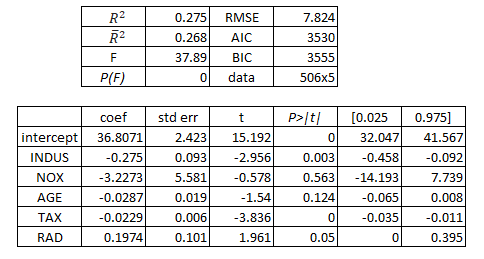
Next, PRICE has been regressed on INDUS, NOX, AGE, TAX, and RAD. In this model, we can see that there are now at least two independent variables that are not statistically significant. The model itself is still significant, but it has a lower F-statistic than the previous model. Additionally, its R2 values are both lower than that of the previous model, implying less explanatory power. RMSE, AIC, and BIC are also higher here, implying lower quality. This confirms the findings calculated above.

接下來，PRICE已針對INDUS，NOX，AGE，TAX和RAD進行了回歸。 在此模型中，我們可以看到，現在至少有兩個獨立變量在統計上不顯著。 該模型本身仍然很重要，但F統計量比以前的模型低。 此外，其R2值均低于先前模型的R2值，這意味著較少的解釋力。 RMSE，AIC和BIC在這里也較高，這意味著質量較低。 這證實了上面計算的結果。

The “z-distance” presented in this blog post has demonstrated its use in this example. The {DIS, RM, PTRATIO, LSTAT, TAX} subset has a shorter distance to 0 than the {INDUS, NOX, AGE, TAX, RAD} subset. DIS, RM, PTRATIO, LSTAT, and TAX were then shown to be better predictors of PRICE. While it was easy to simply fit these two models and compare them, in a feature space of much higher dimension it might be faster to calculate the distances of several subsets.

本博客文章中介紹的“ z -distance”已在示例中證明了其用法。 {DIS，RM，PTRATIO，LSTAT，TAX}子集比{INDUS，NOX，AGE，TAX，RAD}子集的距離短。 然后顯示DIS，RM，PTRATIO，LSTAT和TAX是PRICE的更好預測指標。 盡管很容易簡單地擬合這兩個模型并進行比較，但是在具有更高維度的特征空間中，計算多個子集的距離可能會更快。

結論 (Conclusion)

There are many factors to consider in feature selection. This post does not offer a solution to finding the best subset of variables, but merely a way for one to take a step in the right direction by finding sets of features that do not immediately demonstrate collinearity. It is important to remember that one must rely on more than just correlation coefficients when identifying multicollinearity.

在特征選擇中要考慮許多因素。 這篇文章并沒有提供找到最佳變量子集的解決方案，而只是提供了一種方法，即通過查找未立即證明共線性的特征集，朝正確的方向邁出了一步。 重要的是要記住，在識別多重共線性時，人們不僅要依賴相關系數。

A Python script for this solution and for automating feature combinations can be found at the following GitHub repository:

可在以下GitHub存儲庫中找到此解決方案和自動化功能組合的Python腳本：

https://github.com/willarliss/z-Distance/

https://github.com/willarliss/z-Distance/