Introduction

介紹

In this article, I’d like to speak about linear models by introducing you to a real project that I made. The project that you can find in my Github consists of predicting the prices of fiat 500.

在本文中，我想通過向您介紹我所做的真實項目來談論線性模型。 您可以在我的Github中找到的項目包括預測菲亞特500的價格。

The dataset for my model presents 8 columns as you can see below and 1538 rows.

我的模型的數據集包含8列(如下所示)和1538行。

• model: pop, lounge, sport
  模特：流行，休閑，運動
• engine_power: Kw of the engine
  engine_power：發動機的千瓦
• age_in_days: age of the car in days
  age_in_days：汽車的使用天數
• km: kilometres of the car
  km：汽車的公里數
• previous_owners: number of previous owners
  previous_owners：以前的所有者數
• lat: latitude of the seller (the price of cars in Italy varies from North to South of the country)
  lat：賣方的緯度(意大利的汽車價格從該國的北部到南部不等)
• lon: longitude of the seller (the price of cars in Italy varies from North to South of the country)
  lon：賣方的經度(意大利的汽車價格從該國的北部到南部不等)
• price: selling price
  價格：售價

During this article, we will see in the first part some concepts about the linear regression, the ridge regression and the lasso regression. Then I will show you the fundamental insights that I found about the dataset I considered and last but not least we will see the preparation and the metrics I used to evaluate the performance of my model.

在本文中，我們將在第一部分中看到有關線性回歸，嶺回歸和套索回歸的一些概念。 然后，我將向您展示我對所考慮的數據集的基本見解，最后但并非最不重要的一點是，我們將看到用于評估模型性能的準備工作和度量標準。

Part I: Linear Regression, Ridge Regression and Lasso Regression

第一部分：線性回歸，嶺回歸和套索回歸

Linear models are a class of models that make a prediction using a linear function of the input features.

線性模型是使用輸入要素的線性函數進行預測的一類模型。

For what concerns regression, as we know the general formula looks like as follows:

對于回歸問題，我們知道一般公式如下所示：

As you already know x[0] to x[p] represents the features of a single data point. Instead, m a b are the parameters of the model that are learned and ? is the prediction the model makes.

如您所知，x [0]至x [p]表示單個數據點的特征。 取而代之的是，m是一B是被學習的模型的參數，y是預測的模型使。

There are many linear models for regression. The difference between these models is about how the model parameters m and b are learned from the training data and how model complexity can be controlled. We will see three models for regression.

有許多線性模型可用于回歸。 這些模型之間的差異在于如何從訓練數據中學習模型參數m和b以及如何控制模型復雜性。 我們將看到三種回歸模型。

• Linear regression (ordinary least squares) → it finds the parameters m and b that minimize the mean squared error between predictions and the true regression targets, y, on the training set. The MSE is the sum of the squared differences between the predictions and the true value. Below how to compute it with scikit-learn.

  線性回歸(普通最小二乘) →它找到參數m和b ，該參數使訓練集上的預測與真實回歸目標y之間的均方誤差最小。 MSE是預測值與真實值之間平方差的總和。 下面是如何使用scikit-learn計算它。

from sklearn.linear_model import LinearRegression X_train, X_test, y_train, y_test=train_test_split(X, y, random_state=0)lr = LinearRegression()lr.fit(X_train, y_train)print(“lr.coef_: {}”.format(lr.coef_)) print(“lr.intercept_: {}”.format(lr.intercept_))

• Ridge regression → the formula it uses to make predictions is the same one used for the linear regression. In the ridge regression, the coefficients(m) are chosen for predicting well on the training data but also to fit the additional constraint. We want all entries of m should be close to zero. That means each feature should have a little effect on the outcome as possible(small slope), while still predicting well. This constraint is called regularization which means restricting a model to avoid overfitting. The particular ridge regression regularization is known as L2. Ridge regression is implemented in linear_model.Ridge as you can see below. In particular, by increasing alpha, we move the coefficients toward zero, which decreases training set performance but might help generalization and avoid overfitting.

  Ridge回歸 →用于進行預測的公式與用于線性回歸的公式相同。 在嶺回歸中，選擇系數(m)可以很好地預測訓練數據，但也可以擬合附加約束。 我們希望m的所有條目都應接近零。 這意味著每個特征都應該對結果產生盡可能小的影響(小斜率)，同時仍能很好地預測。 此約束稱為正則化，這意味著限制模型以避免過度擬合。 特定的嶺回歸正則化稱為L2。 Ridge回歸在linear_model.Ridge中實現，如下所示。 特別是，通過增加alpha，我們會將系數移向零，這會降低訓練集的性能，但可能有助于泛化并避免過度擬合。

from sklearn.linear_model import Ridge ridge = Ridge(alpha=11).fit(X_train, y_train)print(“Training set score: {:.2f}”.format(ridge.score(X_train, y_train))) print(“Test set score: {:.2f}”.format(ridge.score(X_test, y_test)))

• Lasso regression → an alternative for regularizing is Lasso. As with ridge regression, using the lasso also restricts coefficients to be close to zero, but in a slightly different way, called L1 regularization. The consequence of L1 regularization is that when using the lasso, some coefficients are exactly zero. This means some features are entirely ignored by the model.

  拉索回歸 →拉索正則化的替代方法。 與ridge回歸一樣，使用套索也將系數限制為接近零，但方式略有不同，稱為L1正則化。 L1正則化的結果是，使用套索時，某些系數正好為零。 這意味著模型將完全忽略某些功能。

from sklearn.linear_model import Lasso lasso = Lasso(alpha=3).fit(X_train, y_train) 
print(“Training set score: {:.2f}”.format(lasso.score(X_train, y_train))) print(“Test set score: {:.2f}”.format(lasso.score(X_test, y_test))) print(“Number of features used: {}”.format(np.sum(lasso.coef_ != 0)))

Part II: Insights that I found

第二部分：我發現的見解

Before to see the part about the preparation and evaluation of the model, it is useful to take a look at the situation of the dataset.

在查看有關模型準備和評估的部分之前，先了解一下數據集的情況是很有用的。

In the below scatter matrix we can observe that there some particular correlations between some features like km, age_in_days and price.

在下面的散點矩陣中，我們可以觀察到某些特征(例如km，age_in_days和價格)之間存在某些特定的相關性。

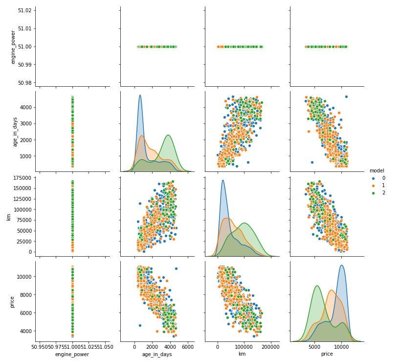
Instead in the following correlation-matrix, we can see very well the result of correlations between the features.

相反，在下面的相關矩陣中，我們可以很好地看到特征之間的相關結果。

In particular, between age_in_days and price or km and price, we have a great correlation.

特別是在age_in_days和價格之間或km和價格之間，我們有很大的相關性。

This is the starting point for constructing our model and know which machine learning model could be fit better.

這是構建我們的模型的起點，并且知道哪種機器學習模型更合適。

Part III: Prepare and evaluate the performance of the model

第三部分：準備和評估模型的性能

To train and test the dataset I used the Linear Regression.

為了訓練和測試數據集，我使用了線性回歸。

from sklearn.linear_model import LinearRegression
X_train, X_test, y_train, y_test = train_test_split(X, y, test_size=0.2, random_state=0)
lr = LinearRegression()
lr.fit(X_train, y_train)

out:

出：

LinearRegression(copy_X=True, fit_intercept=True, n_jobs=None, normalize=False)

In the following table, there are the coefficients for each feature that I considered for my model.

下表列出了我為模型考慮的每個功能的系數。

coef_df = pd.DataFrame(lr.coef_, X.columns, columns=['Coefficient'])
coef_df

out:

出：

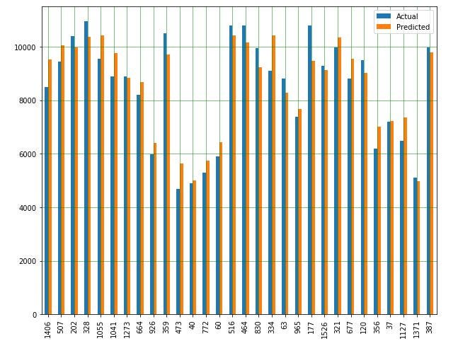
Now, it is time to evaluate the model. In the following graph, characterized by a sample of 30 data points, we can observe the comparison between predicted values and actual values. As we can see our model is pretty good.

現在，該評估模型了。 在以30個數據點為樣本的下圖中，我們可以觀察到預測值與實際值之間的比較。 我們可以看到我們的模型非常好。

The R-squared is a good measure of the ability of the model inputs to explain the variation of the dependent variables. In our case, we have 85%.

R平方可以很好地衡量模型輸入解釋因變量變化的能力。 就我們而言，我們有85％。

from sklearn.metrics import r2_score round(sklearn.metrics.r2_score(y_test, y_pred), 2)

out:

出：

0.85

Now I compute the MAE, MSE and the RMSE to have a more precise overview of the performance of the model.

現在，我計算MAE，MSE和RMSE，以更精確地概述模型的性能。

from sklearn import metrics print(‘Mean Absolute Error:’, metrics.mean_absolute_error(y_test, y_pred)) print(‘Mean Squared Error:’, metrics.mean_squared_error(y_test, y_pred))print(‘Root Mean Squared Error:',
np.sqrt(metrics.mean_squared_error(y_test, y_pred)))

Finally, by comparing the training set score and the test set score we can see how performative is our model.

最后，通過比較訓練集得分和測試集得分，我們可以看到模型的性能如何。

print("Training set score: {:.2f}".format(lr.score(X_train, y_train)))print("Test set score: {:.2f}".format(lr.score(X_test, y_test)))

out:

出：

Training set score: 0.83 Test set score: 0.85

Conclusion

結論

Linear models are a class of models that are widely used in practice and have been studied extensively in the last few years in particular for machine learning. So, with this article, I hope you have obtained a good starting point in order to improve yourself and create your own Linear model.

線性模型是一類在實踐中廣泛使用的模型，并且在最近幾年中，特別是對于機器學習，已經進行了廣泛的研究。 因此，希望本文能夠為您提高自己并創建自己的線性模型提供一個良好的起點。

Thanks for reading this. There are some other ways you can keep in touch with me and follow my work:

感謝您閱讀本文。 您可以通過其他方法與我保持聯系并關注我的工作：

• Subscribe to my newsletter.

  訂閱我的時事通訊。

• You can also get in touch via my Telegram group, Data Science for Beginners.

  您也可以通過我的電報小組“ 面向初學者的數據科學”來聯系 。