by Braden Riggs and George Williams (gwilliams@gsitechnology.com)

Braden Riggs和George Williams(gwilliams@gsitechnology.com)

Whether you are new to the field of data science or a seasoned veteran, you have likely come into contact with the term, ‘nearest-neighbor search’, or, ‘similarity search’. In fact, if you have ever used a search engine, recommender, translation tool, or pretty much anything else on the internet then you have probably made use of some form of nearest-neighbor algorithm. These algorithms, the ones that permeate most modern software, solve a very simple yet incredibly common problem. Given a data point, what is the closest match from a large selection of data points, or rather what point is most like the given point? These problems are “nearest-neighbor” search problems and the solution is an Approximate Nearest Neighbor algorithm or ANN algorithm for short.

無論您是數據科學領域的新手還是經驗豐富的資深人士，您都可能接觸過“最近鄰居搜索”或“相似搜索”一詞。 實際上，如果您曾經使用搜索引擎，推薦器，翻譯工具或互聯網上的幾乎所有其他工具，那么您可能已經在使用某種形式的最近鄰居算法。 這些算法已滲透到大多數現代軟件中，解決了一個非常簡單但難以置信的常見問題。 給定一個數據點，從大量數據點中選擇最接近的匹配是什么 ，或者最像給定點的是哪個點？ 這些問題是“最近鄰居”搜索 問題和解決方案是簡稱為“ 近似最近鄰居”算法或ANN算法。

Approximate nearest-neighbor algorithms or ANN’s are a topic I have blogged about heavily, and with good reason. As we attempt to optimize and solve the nearest-neighbor challenge, ANN’s continue to be at the forefront of elegant and optimal solutions to these problems. Introductory Machine learning classes often include a segment about ANN’s older brother kNN, a conceptually simpler style of nearest-neighbor algorithm that is less efficient but easier to understand. If you aren’t familiar with kNN algorithms, they essentially work by classifying unseen points based on “k” number of nearby points, where the vicinity or distance of the nearby points are calculated by distance formulas such as euclidian distance.

近似最近鄰算法或ANN是我在博客上大量談論的主題，并且有充分的理由。 在我們嘗試優化和解決最鄰近的挑戰時，ANN始終處于解決這些問題的最佳方案的最前沿。 機器學習入門課程通常包括有關ANN的哥哥kNN的部分，kNN是概念上更簡單的近鄰算法樣式，效率較低，但更易于理解。 如果您不熟悉kNN算法，則它們實際上是通過基于“ k”個鄰近點數對看不見的點進行分類來工作的，其中，鄰近點的鄰近度或距離是通過諸如歐幾里得距離的距離公式來計算的。

ANN’s work similarly but with a few more techniques and strategies that ensure greater efficiency. I go into more depth about these techniques in an earlier blog here. In this blog, I describe an ANN as:

ANN的工作與此類似，但是有更多的技術和策略可以確保更高的效率。 我在這里先前的博客中對這些技術進行了更深入的介紹。 在此博客中， 我將ANN描述為 ：

A faster classifier with a slight trade-off in accuracy, utilizing techniques such as locality sensitive hashing to better balance speed and precision.- Braden Riggs, How to Benchmark ANN Algorithms

一種更快的分類器，在精度上會稍有取舍，利用諸如位置敏感的哈希值之類的技術來更好地平衡速度和精度。- Braden Riggs，如何對ANN算法進行基準測試

The problem with utilizing the power of ANNs for your own projects is the sheer quantity of different implementations open to the public, each having their own benefits and disadvantages. With so many choices available how can you pick which is right for your project?

在您自己的項目中使用ANN的功能所帶來的問題是，向公眾開放的不同實現的數量龐大，每個實現都有其自身的優缺點。 有這么多選擇，您如何選擇最適合您的項目？

Bernhardsson和ANN救援基準： (Bernhardsson and ANN-Benchmarks to the Rescue:)

We have established that there are a range of ANN implementations available for use. However, we need a way of picking out the best of the best, the cream of the crop. This is where Aumüller, Bernhardsson, and Faithfull’s paper ANN-Benchmarks: A Benchmarking Tool for Approximate Nearest Neighbor Algorithms and its corresponding GitHub repository comes to our rescue.

我們已經建立了一系列可供使用的ANN實現。 但是，我們需要一種方法來挑選最好的農作物。 這是Aumüller，Bernhardsson和Faithfull的論文ANN基準：近似最近鄰居算法的基準工具 并且其相應的GitHub存儲庫可為我們提供幫助。

The project, which I have discussed in the past, is a great starting point for choosing the algorithm that is the best fit for your project. The paper uses some clever techniques to evaluate the performance of a number of ANN implementations on a selection of datasets. It has these ANN algorithms solve nearest-neighbor queries to determine the accuracy and efficiency of the algorithm at different parameter combinations. The algorithm uses these queries to locate the 10 nearest data points to the queried point and evaluates how close each point is to the true neighbor, which is a metric called Recall. This is then scaled against how quickly the algorithm was able to accomplish its goal, which it called Queries per Second. This metric provides a great reference for determining which algorithms may be most preferential for you and your project.

我過去討論過的項目是選擇最適合您項目的算法的一個很好的起點。 本文使用一些巧妙的技術來評估多種ANN實施對所選數據集的性能。 它具有這些ANN算法來解決最近鄰居查詢，以確定算法在不同參數組合下的準確性和效率。 該算法使用這些查詢來定位到查詢點最近的10個數據點，并評估每個點與真實鄰居的接近程度，這是一個稱為“回叫”的度量。 然后，根據算法能夠實現其目標的速度(稱為“每秒查詢”)進行縮放。 該指標為確定哪種算法可能最適合您和您的項目提供了很好的參考。

Part of conducting this experiment requires picking the algorithms we want to test, and the dataset we want to perform the queries on. Based off of the experiments I have conducted on my previous blogs, narrowing down the selection of algorithms wasn’t difficult. In Bernhardsson’s original project he includes 18 algorithms. Given the performance I had seen in my first blog, using the glove-25 angular natural language dataset, there are 9 algorithms worth considering for our benchmark experiment. This is because some algorithms perform so slowly and so poorly that they aren’t even worth considering in this experiment. The algorithms selected are:

進行此實驗的一部分需要選擇我們要測試的算法，以及我們要對其執行查詢的數據集。 根據我在以前的博客上進行的實驗，縮小算法的選擇范圍并不困難。 在Bernhardsson的原始項目中，他包括18種算法。 鑒于我在第一個博客中看到的性能，使用了Gloves-25角度自然語言數據集，有9種算法值得我們進行基準測試。 這是因為某些算法的執行速度如此之慢且如此差，以至于在本實驗中甚至都不值得考慮。 選擇的算法是：

• Annoy: Spotify's “Approximate Nearest Neighbors Oh Yeah” ANN implementation.

  煩惱： Spotify的 “哦，是，最近的鄰居” ANN實現。

• Faiss: The suite of algorithms Facebook uses for large dataset similarity search including Faiss-lsh, Faiss-hnsw, and Faiss-ivf.

  Faiss： Facebook用于大型數據集相似性搜索的算法套件，包括Faiss-lsh ， Faiss-hnsw和Faiss-ivf 。

• Flann: Fast Library for ANN.

  Flann： ANN的快速庫。

• HNSWlib: Hierarchical Navigable Small World graph ANN search library.

  HNSWlib：分層可導航小世界圖ANN搜索庫。

• NGT-panng: Yahoo Japan’s Neighborhood Graph and Tree for Indexing High-dimensional Data.

  NGT-panng： Yahoo Japan的鄰域圖和樹，用于索引高維數據。

• Pynndescent: Python implementation of Nearest Neighbor Descent for k-neighbor-graph construction and ANN search.

  Pynndescent：用于k鄰域圖構建和ANN搜索的Nearest Neighbor Descent的Python實現。

• SW-graph(nmslib): Small world graph ANN search as part of the non-metric space library.

  SW-graph(nmslib)：小世界圖ANN搜索，作為非度量空間庫的一部分。

In addition to the algorithms, it was important to pick a dataset that would help distinguish the optimal ANN implementations from the not so optimal ANN implementations. For this task, we chose 1% — or a 10 million vector slice — of the gargantuan Deep-1-billion dataset, a 96 dimension computer vision training dataset. This dataset is large enough for inefficiencies in the algorithms to be accentuated and provide a relevant challenge for each one. Because of the size of the dataset and the limited specification of our hardware, namely the 64GBs of memory, some algorithms were unable to fully run to an accuracy of 100%. To help account for this, and to ensure that background processes on our machine didn’t interfere with our results, each algorithm and all of the parameter combinations were run twice. By doubling the number of benchmarks conducted, we were able to average between the two runs, helping account for any interruptions on our hardware.

除算法外，重要的是選擇一個有助于區分最佳ANN實現與非最佳ANN實現的數據集。 為此，我們選擇了龐大的Deep-billion數據集(96維計算機視覺訓練數據集)的1％(即一千萬個矢量切片)。 該數據集足夠大，可以突出算法的低效率，并為每個算法帶來相關挑戰。 由于數據集的大小和我們硬件的有限規格(即64GB內存)，某些算法無法完全運行到100％的精度。 為了解決這個問題，并確保我們機器上的后臺進程不會干擾我們的結果，每種算法和所有參數組合都運行兩次。 通過將執行的基準測試數量加倍，我們可以在兩次運行之間求平均值，從而幫助解決硬件上的任何中斷。

This experiment took roughly 11 days to complete but yielded some helpful and insightful results.

該實驗大約花費了11天的時間，但得出了一些有益而有見地的結果。

我們發現了什么？ (What did we find?)

After the exceptionally long runtime, the experiment completed with only three algorithms failing to fully reach an accuracy of 100%. These algorithms were Faiss-lsh, Flann, and NGT-panng. Despite these algorithms not reaching perfect accuracy, their results are useful and indicate where the algorithm may have been heading if we had experimented with more parameter combinations and didn't exceed memory usage on our hardware.

經過異常長的運行時間后，實驗僅用三種算法就無法完全達到100％的精度。 這些算法是Faiss-lsh ， Flann和NGT-panng 。 盡管這些算法沒有達到完美的精度，但是它們的結果還是有用的，它們表明了如果我們嘗試了更多的參數組合并且未超過硬件上的內存使用量，該算法可能會前進。

Before showing off the results, let’s quickly discuss how we are presenting these results and what terminology you need to understand. On the y-axis, we have Queries per Second or QPS. QPS quantifies the number of nearest-neighbor searches that can be conducted in a second. This is sometimes referred to as the inverse ‘latency’ of the algorithm. More precisely QPS is a bandwidth measure and is inversely proportional to the latency. As the query time goes down, the bandwidth will increase. On the x-axis, we have Recall. In this case, Recall essentially represents the accuracy of the function. Because we are finding the 10 nearest-neighbors of a selected point, the Recall score takes the distances of the 10 nearest-neighbors our algorithms computed and compares them to the distance of the 10 true nearest-neighbors. If the algorithm selects the correct 10 points it will have a distance of zero from the true values and hence a Recall of 1. When using ANN algorithms we are constantly trying to maximize both of these metrics. However, they often improve at each other’s expense. When you speed up your algorithm, thereby improving latency, it becomes less accurate. On the other hand, when you prioritize its accuracy, thereby improving Recall, the algorithm slows down.

在展示結果之前，讓我們快速討論一下我們如何呈現這些結果以及您需要了解哪些術語。 在y軸上，我們有每秒查詢數或QPS。 QPS量化了每秒可以進行的最近鄰居搜索的次數。 有時將其稱為算法的逆“潛伏期”。 更準確地說，QPS是帶寬量度，與延遲成反比。 隨著查詢時間的減少，帶寬將增加。 在x軸上，我們有Recall 。 在這種情況下，調用實質上代表了函數的準確性。 由于我們正在查找選定點的10個最近鄰居，因此Recall分數將采用我們的算法計算出的10個最近鄰居的距離，并將它們與10個真實最近鄰居的距離進行比較。 如果該算法選擇了正確的10個點，則它與真實值的距離為零，因此召回率為1。使用ANN算法時，我們一直在努力使這兩個指標最大化。 但是，它們通常會以互相犧牲為代價而有所改善。 當您加快算法速度從而改善延遲時，它的準確性就會降低。 另一方面，當您優先考慮其準確性從而提高查全率時，該算法會變慢。

Pictured below is the plot of Queries Performed per Second, over the Recall of the algorithm:

下圖是算法調用時每秒執行的查詢的圖：

As evident by the graph above there were some clear winners and some clear losers. Focusing on the winners, we can see a few algorithms that really stand out, namely HNSWlib (yellow) and NGT-panng (red) both of which performed at a high accuracy and a high speed. Even though NGT never finished, the results do indicate it was performing exceptionally well prior to a memory-related failure.

從上圖可以明顯看出，有一些明顯的贏家和一些明顯的輸家。 著眼于獲勝者，我們可以看到一些真正脫穎而出的算法，即HNSWlib(黃色)和NGT-panng(紅色)，它們均以高精度和高速執行。 盡管NGT從未完成，但結果確實表明它在與內存相關的故障之前表現出色。

So given these results, we now know which algorithms to pick for our next project right?

因此，鑒于這些結果，我們現在知道為下一個項目選擇哪種算法對嗎？

Unfortunately, this graph doesn’t depict the full story when it comes to the efficiency and accuracy of these ANN implementations. Whilst HNSWlib and NGT-panng can perform quickly and accurately, that is only after they have been built. “Build time” refers to the length of time that is required for the algorithm to construct its index and begin querying neighbors. Depending on the implementation of the algorithm, build time can be a few minutes or a few hours. Graphed below is the average algorithm build time for our benchmark excluding Faiss-HNSW which took 1491 minutes to build (about 24 hours):

不幸的是，當涉及到這些ANN實現的效率和準確性時，該圖并沒有完整描述。 雖然HNSWlib和NGT-panng可以快速而準確地執行，但這只是在它們構建之后。 “構建時間”是指算法構建其索引并開始查詢鄰居所需的時間長度。 根據算法的實現，構建時間可能是幾分鐘或幾小時。 下圖是我們的基準測試的平均算法構建時間， 不包括Faiss-HNSW，該過程花費了1491分鐘的構建時間(約24小時) ：

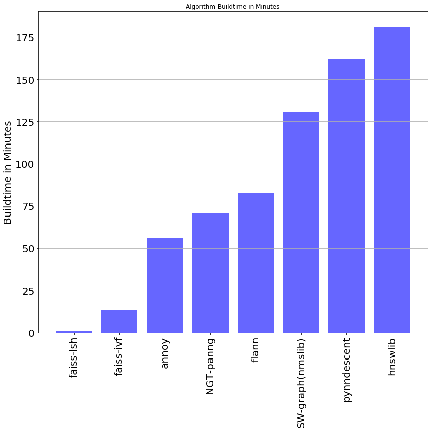
As we can see the picture changes substantially when we account for the time spend “building” the algorithm’s indexes. This index is essentially a roadmap for the algorithm to follow on its journey to find the nearest-neighbor. It allows the algorithm to take shortcuts, accelerating the time taken to find a solution. Depending on the size of the dataset and how intricate and comprehensive this roadmap is, build-time can be between a matter of seconds and a number of days. Although accuracy is always a top priority, depending on the circumstances it may be advantageous to choose between algorithms that build quickly or algorithms that run quickly:

正如我們看到的那樣，當我們考慮“構建”算法索引所花費的時間時，情況會發生很大的變化。 該索引本質上是該算法在查找最近鄰居的過程中要遵循的路線圖。 它允許算法采用快捷方式，從而加快了找到解決方案的時間。 根據數據集的大小以及此路線圖的復雜程度，構建時間可能在幾秒鐘到幾天之間。 盡管準確性始終是頭等大事，但根據具體情況，在快速構建的算法或快速運行的算法之間進行選擇可能會比較有利：

• Scenario #1: You have a dataset that updates regularly but isn’t queried often, such as a school’s student attendance record or a government’s record of birth certificates. In this case, you wouldn’t want an algorithm that builds slowly because each time more data is added to the set, the algorithm must rebuild it’s index to maintain a high accuracy. If your algorithm builds slowly this could waste valuable time and energy. Algorithms such as Faiss-IVF are perfect here because they build fast and are still very accurate.

  場景1：您有一個定期更新但不經常查詢的數據集，例如學校的學生出勤記錄或政府的出生證明記錄。 在這種情況下，您不希望算法構建緩慢，因為每次將更多數據添加到集合中時，該算法必須重建其索引以保持較高的準確性。 如果算法構建緩慢，可能會浪費寶貴的時間和精力。 Faiss-IVF之類的算法在這里非常理想，因為它們構建速度很快并且仍然非常準確。

• Scenario #2: You have a static dataset that doesn’t change often but is regularly queried, like a list of words in a dictionary. In this case, it is more preferential to use an algorithm that is able to perform more queries per second, at the expense of built time. This is because we aren’t adding new data regularly and hence don’t need to rebuild the index regularly. Algorithms such as HNSWlib or NGT-panng are perfect for this because they are accurate and fast, once the build is completed.

  場景2：您有一個靜態數據集，該數據集不會經常更改，而是會定期查詢，例如字典中的單詞列表。 在這種情況下，更可取的是使用能夠每秒執行更多查詢的算法，但會浪費構建時間。 這是因為我們不會定期添加新數據，因此不需要定期重建索引。 HNSWlib或NGT-panng之類的算法非常適合此操作，因為一旦構建完成，它們便準確且快速。

There is a third scenario worth mentioning. In my experiments attempting to benchmark ANN algorithms on larger and larger portions of the deep1b dataset, available memory started to become a major limiting factor. Hence, picking an algorithm with efficient use of memory can be a major advantage. In this case, I would highly recommend the Faiss suite of algorithms which have been engineered to perform under some of the most memory starved conditions.

還有第三種情況值得一提。 在我的實驗中，試圖在Deep1b數據集的越來越大的部分上對ANN算法進行基準測試 ，可用內存開始成為主要的限制因素。 因此，選擇一種有效利用內存的算法可能是一個主要優勢。 在這種情況下，我強烈建議使用Faiss算法套件，這些套件經設計可在某些內存不足的情況下執行。

Regardless of the scenario, we almost always want high accuracy. In our case accuracy, or recall, is evaluated based on the algorithm’s ability to correctly determine the 10 nearest-neighbors of a given point. Hence the algorithm’s performance could change if we consider its 100 nearest-neighbors or its single nearest-neighbor.

無論哪種情況，我們幾乎總是希望獲得高精度。 在我們的情況下，根據算法正確確定給定點的10個最近鄰居的能力來評估準確性或召回率。 因此，如果我們考慮它的100個最近鄰居或單個最近鄰居，算法的性能可能會改變。

摘要： (The Summary:)

Based on our findings from this benchmark experiment there are clear benefits to using some algorithms as opposed to others. The key to picking an optimal ANN algorithm is understanding what about the algorithm you want to prioritize and what engineering tradeoffs you are comfortable with. I recommend you prioritize what fits your circumstances, be that speed (QPS), accuracy (Recall), or pre-processing (Build time). It is worth noting algorithms that perform with less than 90% Recall aren’t worth discussing. This is because 90% is considered to be the minimum level of performance when conducting nearest-neighbor search. Anything less than 90% is underperforming and likely not useful.

根據我們從基準測試中獲得的發現，使用某些算法相對于其他算法具有明顯的好處。 選擇最佳ANN算法的關鍵是了解要確定優先級的算法是什么，以及需要進行哪些工程折衷。 我建議您優先考慮適合您的情況的速度，即速度(QPS)，準確性(調用)或預處理(構建時間)。 值得注意的是，調用率不到90％的算法不值得討論。 這是因為在執行最近鄰居搜索時，90％被認為是最低性能。 少于90％的廣告效果不佳，可能沒有用。

With that said my recommendations are as follows:

話雖如此，我的建議如下：

• For projects where speed is a priority, our results suggest that algorithms such as HNSWlib and NGT-panng perform accurately with a greater number of queries per second than alternative choices.

  對于優先考慮速度的項目，我們的結果表明，與其他選擇相比，諸如HNSWlib和NGT-panng之類的算法每秒執行的查詢數量更高， 因此能夠準確執行。

• For Projects where accuracy is a priority, our results suggest that algorithms such as Faiss-IVF and SW-graph prioritize higher Recall scores, whilst still performing quickly.

  對于以準確性為優先的項目，我們的結果表明，諸如Faiss-IVF和SW-graph之類的算法會優先考慮較高的查全率，同時仍能快速執行。

• For projects where pre-processing is a priority, our results suggest that algorithms such as Faiss-IVF and Annoy exhibit exceptionally fast build times whilst still balancing accuracy and speed.

  對于需要優先處理的項目，我們的結果表明，諸如Faiss-IVF和Annoy之類的算法顯示出異常快的構建時間，同時仍然在準確性和速度之間取得了平衡。

Considering the circumstances of our experiment, there are a variety of different scenarios where some algorithms may perform better than others. In our case, we have tried to perform in the most generic and common of circumstances. We used a large dataset with high, but not excessively high, dimensionality to help indicate how these algorithms may perform on sets with similar specifications. For some of these algorithms, more tweaking and experimentation may lead to marginal improvements in runtime and accuracy. However, given the scope of this project it would be excessive to attempt to accomplish this with each algorithm.

考慮到我們的實驗環境，在許多不同的情況下，某些算法的性能可能會優于其他算法。 在我們的案例中，我們試圖在最普通和最常見的情況下執行。 我們使用了一個具有高(但不是過高)維的大型數據集，以幫助指示這些算法如何在具有相似規格的集合上執行。 對于其中一些算法，更多的調整和實驗可能會導致運行時和準確性的輕微改善。 但是，鑒于該項目的范圍，嘗試使用每種算法來完成此任務將是多余的。

If you are interested in learning more about Bernhardsson’s project I recommend reading some of my other blogs on the topic. If you are interested in looking at the full CSV file of results from this benchmark, it is available on my GitHub here.

如果您有興趣了解有關Bernhardsson的項目的更多信息，建議閱讀我有關該主題的其他博客。 如果您有興趣查看此基準測試結果的完整CSV文件，請在我的GitHub上此處獲取 。

未來的工作： (Future Work:)

Whilst this is a good starting point for picking ANN algorithms there are still a number of alternative conditions to consider. Going forward I would like to explore how batch performance impacts our results and whether different algorithms perform better when batching is included. Additionally, I suspect that some algorithms will perform better when querying for different numbers of nearest-neighbors. In this project, we chose 10 nearest neighbors, however, our results could shift when querying for 100 neighbors or just the top 1 nearest-neighbor.

雖然這是選擇ANN算法的一個很好的起點，但仍然需要考慮許多替代條件。 展望未來，我想探討批處理性能如何影響我們的結果以及包括批處理時不同算法的性能是否更好。 另外，我懷疑在查詢不同數量的最近鄰居時某些算法的性能會更好。 在該項目中，我們選擇了10個最近的鄰居，但是，當查詢100個鄰居或僅搜索前1個最近的鄰居時，結果可能會發生變化。

附錄： (Appendix:)

1. Computer specifications: 1U GPU Server 1 2 Intel CD8067303535601 Xeon? Gold 5115 2 3 Kingston KSM26RD8/16HAI 16GB 2666MHz DDR4 ECC Reg CL19 DIMM 2Rx8 Hynix A IDT 4 4 Intel SSDSC2KG960G801 S4610 960GB 2.5" SSD.

   計算機規格： 1U GPU服務器1 2 Intel CD8067303535601Xeon?Gold 5115 2 3 Kingston KSM26RD8 / 16HAI 16GB 2666MHz DDR4 ECC Reg CL19 DIMM 2Rx8 Hynix A IDT 4 4 Intel SSDSC2KG960G801 S4610 960GB 2.5“ SSD。

2. Link to How to Benchmark ANN Algorithms: https://medium.com/gsi-technology/how-to-benchmark-ann-algorithms-a9f1cef6be08

   鏈接到如何對ANN算法進行基準測試： https : //medium.com/gsi-technology/how-to-benchmark-ann-algorithms-a9f1cef6be08

3. Link to ANN Benchmarks: A Data Scientist’s Journey to Billion Scale Performance: https://medium.com/gsi-technology/ann-benchmarks-a-data-scientists-journey-to-billion-scale-performance-db191f043a27

   鏈接到ANN基準：數據科學家的十億規模績效之旅： https : //medium.com/gsi-technology/ann-benchmarks-a-data-scientists-journey-to-billion-scale-performance-db191f043a27

4. Link to CSV file that includes benchmark results: https://github.com/Briggs599/Deep1b-benchmark-results

   鏈接到包含基準測試結果的CSV文件： https : //github.com/Briggs599/Deep1b-benchmark-results

資料來源： (Sources:)

1. Aumüller, Martin, Erik Bernhardsson, and Alexander Faithfull. “ANN-benchmarks: A benchmarking tool for approximate nearest neighbor algorithms.” International Conference on Similarity Search and Applications. Springer, Cham, 2017.

   Aumüller，Martin，Erik Bernhardsson和Alexander Faithfull。 “ ANN基準：用于近似最近鄰算法的基準測試工具。” 國際相似性搜索及其應用會議 。 占卜·斯普林格，2017年。

2. Deep billion-scale indexing. (n.d.). Retrieved July 21, 2020, from http://sites.skoltech.ru/compvision/noimi/

   十億規模的深索引。 (nd)。 于2020年7月21日從http://sites.skoltech.ru/compvision/noimi/檢索

3. Liu, Ting, et al. “An investigation of practical approximate nearest neighbor algorithms.” Advances in neural information processing systems. 2005.

   劉婷，等。 “研究實用的近似最近鄰算法。” 神經信息處理系統的研究進展 。 2005。