As a Data Scientist, I spend quite a bit of time thinking about Customer Lifetime Value (CLV) and how to model it. A strong CLV model is really a strong customer behavior model — the better you can predict next actions, the better you can quantify CLV.

作為數據科學家，我花了很多時間思考客戶生命周期價值(CLV)以及如何對其建模。 強大的CLV模型實際上是強大的客戶行為模型-您可以更好地預測下一步行動，就可以更好地量化CLV。

In this post, I hope to demonstrate, through both a toy and real-world example, why using aggregate statistics to judge the strength of a customer behavior model is a bad idea.

在本文中，我希望通過一個玩具實例和一個真實示例來說明為什么使用匯總統計數據來判斷客戶行為模型的優勢是一個壞主意 。

Instead, the best CLV Model is the one that has the strongest predictions on the individual level. Data Scientists exploring Customer Lifetime Value should primarily, and perhaps only, use individual level metrics to fully understand the strengths and weaknesses of a CLV model.

相反，最好的CLV模型是在單個級別上具有最強預測的模型。 探索客戶生命周期價值的數據科學家應主要(也許僅)使用個人級別的指標來全面了解CLV模型的優缺點。

第1章什么是CLV，為什么重要？ (Ch.1 What is CLV, and why is it important?)

While this is intended for Data Scientists, I wanted to address the business ramifications of this article, since understanding the business need will inform both why I hold certain opinions and why it is important for all of us to grasp the added benefit of a good CLV model.

雖然這是供數據科學家使用的，但我想解決本文的業務問題，因為了解業務需求將同時說明我為什么持有某些意見以及為什么對所有人來說，掌握良好CLV的額外好處很重要模型。

CLV: How much a customer will spend in the future

CLV ：客戶將來會花費多少

CLV is a business KPI that has exploded in popularity over the past few years. The reason is obvious: if your company can accurately predict how much a customer will spend over the next couple months or years, you can tailor their experience to fit that budget. This has dramatic applications from marketing to customer service to overall business strategy.

CLV是一個業務KPI，在過去幾年中Swift普及。 原因很明顯：如果您的公司可以準確預測客戶在未來幾個月或幾年內的支出，則可以根據預算調整他們的經驗。 從營銷到客戶服務再到整體業務戰略，這都有著引人注目的應用。

Here a quick list of business applications that accurate CLV can help empower:

以下是準確CLV可以幫助實現的業務應用程序的快速列表：

• Marketing Audience Generation
  營銷受眾生成
• Cohort Analysis
  隊列分析
• Customer Service Ticket Ordering
  客戶服務票務訂購
• Marketing Lift Analysis
  營銷提升分析
• CAC bid capping marketing
  CAC出價上限營銷
• Discount Campaigns
  折扣活動
• VIP buying experiences
  VIP購買體驗
• Loyalty Programs
  會員計劃
• Segmentation
  分割
• Board Reporting
  董事會報告

There’s plenty more, these are just the ones that come to my mind the fastest.

還有更多，這些只是我想到的最快的。

With so much business planning at stake, tech-savvy companies are busy scrambling to find which model can best capture CLV of their customer base. The most popular and commonly used customer lifetime value models benchmark their strength on aggregate metrics, using statistics like aggregate revenue percent error (ARPE). I know this because first hand many of my clients have compared their internal CLV models to mine using aggregate statistics.

面對如此多的業務計劃，精通技術的公司正忙于尋找哪種模型最能抓住其客戶群的CLV。 最流行和最常用的客戶生命周期價值模型使用諸如總收入百分比誤差(ARPE)之類的統計數據來衡量其在總指標上的優勢。 我知道這一點是因為第一手資料我的許多客戶已使用匯總統計數據將其內部CLV模型與我的模型進行比較。

I would argue that is a serious mistake.

我認為這是一個嚴重的錯誤。

The following 2 examples, one toy and one real, will hopefully demonstrate how aggregate statistics can both lead us astray and hide model shortcomings that are glaringly apparent at the individual level. This is especially prescient because most business use cases require a strong CLV model at the individual level, not just at the aggregate.

以下兩個示例(一個玩具和一個真實玩具)將有望展示總體統計信息如何使我們誤入歧途并掩蓋模型缺陷，這些缺陷在個人層面上顯而易見。 這是特別有先見之明的，因為大多數業務用例需要在單個級別(而不只是在總體級別)上使用強大的CLV模型。

第2章玩具示例 (Ch.2 A Toy Example)

When you rely on aggregate metrics and ignore the individual-level inaccuracies, you are missing a large part of the technical narrative. Consider the following example of 4 customers and their 1 year CLV:

當您依靠匯總指標并忽略個人級別的不準確性時，您會丟失很大一部分技術敘述。 考慮以下4個客戶及其1年CLV的示例：

This example includes high, low, and medium CLV customers, as well as a churned customer, creating a nice distribution for a smart model to capture.

該示例包括高，低和中級CLV客戶以及攪拌過的客戶，從而為智能模型的捕獲創建了良好的分布。

Now, consider the following validation metrics:

現在，請考慮以下驗證指標：

1. MAE: Mean absolute error (The Average Difference between predictions)

   MAE ：平均絕對誤差(預測之間的平均差)

3. ARPE: Aggregate revenue percent error (The overall difference between total revenue and predicted revenue)

3. ARPE ：總收入百分比誤差(總收入與預期收入之間的總差)

MAE and is on the customer level, while ARPE and is an aggregate statistic. The lower the value for these validation metrics, the better.

MAE和處于客戶級別，而ARPE和處于匯總統計。 這些驗證指標的值越低越好。

This example will demonstrate how an aggregate statistic can bury the shortcomings of low-quality models.

此示例將演示匯總統計信息如何掩蓋低質量模型的缺點。

To do so, compare a dummy guessing the mean to a CLV model off by 20% across the board.

為此，將假想平均數的假人與CLV模型進行比較，將其平均減少20％。

Model 1: The Dummy

模型1：假人

The dummy model will only guess $40 for every customer.

虛擬模型只會為每個客戶猜測$ 40。

Model 2: CLV Model

模型2：CLV模型

This model tries to make an accurate model prediction at the customer level.

該模型試圖在客戶級別做出準確的模型預測。

We can use these numbers to calculate the three validation metrics.

我們可以使用這些數字來計算三個驗證指標。

This example illustrates that a model that is considerably worse in the aggregate (the CLV model is worse by over 20%) is actually better at the individual level.

此示例說明，總體上較差的模型(CLV模型的差值超過20％)實際上在單個級別上更好。

To make this example even better, let’s add some noise to the predictions.

為了使這個示例更好，讓我們在預測中添加一些噪點。

# Dummy Sampling:
# randomly sampling a normal dist around $40 with a SD of $5np.random.normal (40,5,4)OUT: (44.88, 40.63, 40.35, 42.16)#CLV Sampling:
# randomly sampling a normal dist around answer with a SD of $15
max (0, np.random.normal (0,15)),
max (0, np.random.normal (10, 15)),
max (0, np.random.normal (50,15)),
max  (0, np.random.normal (100, 15))OUT: (0, 17.48, 37.45, 81.41)

The results above indicate that even if an individual stat is a higher percentage than you would hope, the distribution of those CLV numbers is more in light with what we are looking for: a model that distinguishes high CLV customers from low CLV customers. If you only look at the aggregate metrics for a CLV model, you are missing a major part of the story, and you may end up choosing the wrong model for your business.

上面的結果表明，即使單個統計數據的百分比超出您的期望，這些CLV編號的分布也更加符合我們的需求：該模型將CLV高客戶與低CLV客戶區分開。 如果僅查看CLV模型的匯總指標，則可能會遺漏故事的大部分內容，最終可能會為您的業務選擇錯誤的模型。

But even rolling up an error metric calculated at the individual level, such as MAE or alternatives like MAPE, can hide critical information about the strengths and weaknesses of your model. Mainly, its capacity to create an accurate distribution of CLV scores.

但是，即使匯總按單個級別計算的誤差度量標準(例如MAE或MAPE等替代方案)，也可能隱藏有關模型優缺點的關鍵信息。 主要是其創建CLV分數的準確分布的能力。

To explore this further, let’s move to a more realistic example

為了進一步探討這一點，讓我們來看一個更現實的例子

第3章一個真實的例子 (Ch.3 A Real Example)

Congratulations! You, the Reader, have been hired as a Data Scientist by BottleRocket Brewing Co, an eCommerce company I just made up. (The data we will use is based on a real eCommerce company that I scrubbed for this post)

恭喜你！ 您(讀者)已被我剛剛組建的電子商務公司BottleRocket Brewing Co聘為數據科學家。 (我們將使用的數據基于我為這篇文章整理的一家真正的電子商務公司)

Your first task as a Data Scientist: Choose the best CLV model for BottleRocket’s business…

作為數據科學家的首要任務：為BottleRocket的業務選擇最佳的CLV模型…

…but what does “best” mean?

…但是“最佳”是什么意思？

Undeterred, you run an experiment with the following models:

不用擔心，您可以使用以下模型進行實驗：

1. Pareto/NBD Model (PNBD)

   帕累托/ NBD模型(PNBD)

The Pareto/NBD model is a very popular choice, and is the model under the hood of most data-driven CLV predictions today. To quote the documentation:

Pareto / NBD模型是一個非常受歡迎的選擇，并且是當今大多數數據驅動的CLV預測的模型。 引用文檔：

The Pareto/NBD model, introduced in 1987, combines the [Negative Binomial Distribution] for transactions of active customers with a heterogeneous dropout process, and to this date can still be considered a gold standard for buy-till-you-die models [Link]

1987年引入的Pareto / NBD模型將活躍客戶交易的[負二項式分布]與異構退出過程結合在一起，到目前為止，仍可以認為是“買到賣-買-買”模型的黃金標準 [Link ]

But another way, the model learns two distributions, one for churn probability and the other for inter transaction-time (ITT) and makes CLV predictions by sampling from these distributions.

但是另一種方法是，該模型學習兩種分布，一種用于流失概率，另一種用于交易間時間(ITT)，并通過從這些分布進行采樣來進行CLV預測。

** Describing BTYD models in more technical detail is a bit out of scope of this article, which is focused on error metrics. Please drop a comment if you are interested in a more in-depth write-up about BTYD models and I’m happy to write a follow-on article!

**更詳細地描述BTYD模型在本文的范圍之內，本文的重點是錯誤度量。 如果您對BTYD模型的更深入的撰寫感興趣，請發表評論，我很樂意寫一篇后續文章！

2. Gradient Boosted Machines (GBM)

2.梯度提升機(GBM)

Gradient Boosted Machines models are a popular machine learning model in which weak trees are trained and assembled together to make a strong overall classifier.

梯度提升機器模型是一種流行的機器學習模型，其中將弱樹訓練并組裝在一起以構成一個強大的整體分類器。

** As with BTYD models, I won’t go into detail about how GBMs work but once again comment below if you’d like me to write up something on method/models

**與BTYD模型一樣，我不會詳細介紹GBM的工作原理，但是如果您希望我在方法/模型上寫點東西，請在下面再次評論

3. Dummy CLV

3.虛擬CLV

This model is defined as simply:

該模型的定義很簡單：

Calculate the average ITT for the business
Calculate the average spend over 1yrIf someone has not bought within 2x the average purchase time:
    Predict $0
Else:
    Predict the average 1y spend

4. Very Dumb Dummy Model (Avg Dummy)

4.非常笨拙的虛擬模型(平均虛擬模型)

This model only guesses the average spend over 1yr for all customers. Included as a baseline for model performance

此模型僅猜測所有客戶在1年以上的平均支出。 作為模型性能的基準

Ch.3.1 The Aggregate Metrics

第3.1章匯總指標

We can consolidate all of these models’ predictions into a nice little Pandas DataFrame `combined_result_pdf` that looks like:

我們可以將所有這些模型的預測合并為一個漂亮的小熊貓DataFrame`combined_result_pdf`，如下所示：

combined_result_pdf.head()

Given this customer table, we can calculate error metrics using the following code:

給定此客戶表，我們可以使用以下代碼來計算錯誤指標：

from sklearn.metrics import mean_absolute_erroractual = combined_result_pdf['actual']
rev_actual = sum(actual)for col in combined_result_pdf.columns:
    if col in ['customer_id', 'actual']:
        continue
    pred = combined_result_pdf[col]
    mae = mean_absolute_error(y_true=actual, y_pred=pred)
    print(col + ": ${:,.2f}".format(mae))
    
    rev_pred = sum(pred)
    perc = 100*rev_pred/rev_actual
    print(col + ": ${:,} total spend ({:.2f}%)".format(pred, perc))

With these four models, we tried to predict 1yr CLV for BottleRocket customers, ranked by MAE score:

對于這四種模型，我們嘗試通過MAE得分對BottleRocket客戶預測1年CLV：

Here are some interesting insights from this table:

下表列出了一些有趣的見解：

1. GBM appears to be the best model for CLV
   GBM似乎是CLV的最佳模型
2. PNBD, despite being a popular CLV, seems to be the worst. In fact, it’s worse than a simple if/else rule list, and only slightly better than a model only guesses the mean!
   盡管PNBD是受歡迎的CLV，但它似乎是最糟糕的。 實際上，它比簡單的if / else規則列表還差，并且僅比模型僅猜測均值好一點！
3. Despite GBM being the best, it’s only a few dollars better than a dummy if/else rule list model
   盡管GBM是最好的，但僅比虛擬if / else規則列表模型好幾美元

Point #3 especially has some interesting ramifications if the Data Scientist/Client accepts it. If the interpreter of these results actually believes that a simple if/else model can capture nearly all the complexity a GBM could capture, and better than the commonly used PNBD model, then obviously the “best” model would be the Dummy CLV once cost, speed of training, and interpretability are all factored in.

如果數據科學家/客戶接受，第3點尤其會產生一些有趣的后果。 如果這些結果的解釋者實際上認為，簡單的if / else模型可以捕獲GBM可以捕獲的幾乎所有復雜性，并且比常用的PNBD模型更好，那么顯然，“最好的”模型是Dummy CLV，一旦投入使用，培訓的速度和可解釋性都是因素。

This brings us back to the original claim — that aggregate error metrics, even ones calculated on the individual level, hide some shortcomings of models. To demonstrate this, let’s rework our DataFrame into Confusion Matrices.

這使我們回到了最初的主張— 聚合錯誤度量標準，即使是在單個級別上計算出的誤差度量標準，也隱藏了模型的某些缺點。 為了證明這一點，讓我們將我們的DataFrame重做為混淆矩陣。

Mini Chapter: What is a Confusion Matrix?

迷你章節：什么是混淆矩陣？

From its name alone, understanding a confusion matrix sounds confusing & challenging. But it is crucial to understand the points being made in this post, as well as a powerful tool to add to your Data Science toolkit.

僅從其名稱來看，理解混淆矩陣聽起來就令人困惑和挑戰。 但是，至關重要的是要了解本文中提出的要點以及將其添加到數據科學工具包中的強大工具。

A Confusion Matrix is a table that outlines the accuracy of classification, and what misclassifications are common by the model. A simple confusion matrix may look like this:

混淆矩陣是一個表格，概述了分類的準確性以及該模型常見的錯誤分類。 一個簡單的混淆矩陣可能看起來像這樣：

The diagonal on the above confusion matrix, highlighted Green, reflects correct predictions — predicting Cat when the it was actually a Cat etc. The rows will add up to 100%, allowing us to get a nice snapshot of how well our model captures Recall behavior, or the probability our model guesses correctly given a specific label.

上面混淆矩陣上的對角線(突出顯示為綠色)反映了正確的預測-預測Cat實際上是Cat等時的行數。這些行的總和為100％，使我們可以很好地捕獲模型捕獲召回行為的方式，或我們的模型在給定特定標簽的情況下正確猜測的可能性。

What we can also tell from the above confusion matrix is..

從上面的混淆矩陣中我們還可以看出。

1. The model is excellent at predicting Cat given the true label is Cat (Cat Recall is 90%)
   該模型非常適合預測Cat，因為真實標簽為Cat(Cat召回率為90％)
2. The model has a difficult time distinguishing between Dogs and Cats, often misclassifying Dogs for Cats. This is the most common mistake made by the model.
   該模型很難區分狗和貓，經常將狗歸為貓。 這是模型最常見的錯誤。
3. While it sometimes misclassifies a Cat as a Dog, it is far less common than other errors
   盡管有時會將貓誤分類為狗，但它比其他錯誤少見

With this in mind, let’s explore how well our CLV models capture customer behavior using Confusion Matrices. A strong model would be able to correctly classify low value customers and high value customers as such. I prefer this method of visualization as opposed to something like a histogram of CLV scores because it reveals what elements of modelling the distribution are the strong and weak.

考慮到這一點，讓我們探究我們的CLV模型如何使用混淆矩陣來捕獲客戶行為。 強大的模型將能夠正確地將低價值客戶和高價值客戶分類。 我喜歡這種可視化方法，而不是像CLV得分的直方圖那樣，因為它揭示了建模分布的要素是強項還是弱項。

To achieve this, we will convert our monetary value predictions into quantiled CLV predictions of Low Medium High and Best. These will be drawn from the quantiles generated by each model’s predictions.

為了實現這一目標，我們將把貨幣價值預測轉換為低中高和最佳的量化CLV預測。 這些將從每個模型的預測生成的分位數中得出。

The best model will correctly categorize customers into these 4 buckets of low/medium/high/best. Therefore each model we will make a confusion matrix of the following structure:

最佳模型將正確地將客戶分類為這4個低/中/高/最佳桶。 因此，每個模型我們都將構成以下結構的混淆矩陣：

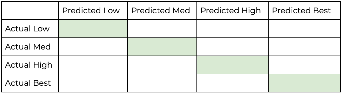
And the best model will have the most amount of predictions that fall within this diagonal.

最好的模型將在此對角線范圍內具有最多的預測。

Ch. 3.2 The Individual Metrics

頻道 3.2個人指標

These confusion matrices can be generated from our Pandas DF with the following code snippet:

這些混淆矩陣可以由我們的Pandas DF使用以下代碼段生成：

from sklearn.metrics import confusion_matrix
import matplotlib.patches as patches
import matplotlib.colors as colors# Helper function to get quantiles
def get_quant_list(vals, quants):
    actual_quants = []
    
    for val in vals:
        if val > quants[2]:
            actual_quants.append(4)
        elif val > quants[1]:
            actual_quants.append(3)
        elif val > quants[0]:
            actual_quants.append(2)
        else:
            actual_quants.append(1)
    return(actual_quants)# Create Plot
fig, axes = plt.subplots(nrows=int(num_plots/2)+(num_plots%2),ncols=2, figsize=(10,5*(num_plots/2)+1))fig.tight_layout(pad=6.0)
tick_marks = np.arange(len(class_names))
plt.setp(axes, xticks=tick_marks, xticklabels=class_names, yticks=tick_marks, yticklabels=class_names)# Pick colors
cmap = plt.get_cmap('Greens')# Generate Quant Labels
plt_num = 0
for col in combined_result_pdf.columns:
    if col in ['customer_id', 'actual']:
        continue
    quants = combined_result_pdf[col]quantile(q=[0.25,0.5,0.75])
    pred = combined_result_pdf[col]
    pred_quants = get_quant_list(pred,quants)
    
    # Generate Conf Matrix
    cm = confusion_matrix(y_true=actual_quants, y_pred=pred_quants)
    ax = axes.flatten()[plt_num]
    accuracy = np.trace(cm) / float(np.sum(cm))
    misclass = 1 - accuracy
     # Clean up CM code
    cm = cm.astype('float') / cm.sum(axis=1)[:, np.newaxis] *100
    ax.imshow(cm, interpolation='nearest', cmap=cmap)
    ax.set_title('{} Bucketting'.format(col))
    thresh = cm.max() / 1.5
 
    for i, j in itertools.product(range(cm.shape[0]), range(cm.shape[1])):        ax.text(j, i, "{:.0f}%".format(cm[i, j]), horizontalalignment="center", color="white" if cm[i, j] > thresh else "black")
 
    # Clean Up Chart
    ax.set_ylabel('True label')
    ax.set_xlabel('Predicted label')
    ax.set_title('{}\naccuracy={:.0f}%'.format(col,100*accuracy))
    ax.spines['top'].set_visible(False)
    ax.spines['right'].set_visible(False)
    ax.spines['bottom'].set_visible(False)
    ax.spines['left'].set_visible(False)
    for i in [-0.5,0.5,1.5,2.5]:
        ax.add_patch(patches.Rectangle((i,i),
        1,1,linewidth=2,edgecolor='k',facecolor='none'))    plt_num += 1

This produces the following Charts:

這將產生以下圖表：

The coloring of the chart is how concentrated a certain prediction/actual classification is — the darker green, the more examples that fall within that square.

圖表的顏色是某個預測/實際分類的集中程度-綠色越深，該正方形內的示例越多。

As with the example confusion matrix discussed above, the diagonal (highlighted with black lines) indicates appropriate classification of customers.

與上面討論的示例混淆矩陣一樣，對角線(用黑線突出顯示)指示適當的客戶分類。

Ch.3.3: Analysis

第3.3章：分析

Dummy Models (Top Row)

虛擬模型(頂行)

Dummy1, which is only predicting the average every time, has a distribution of ONLY the mean. It makes no distinction between high or low value customers.

Dummy1每次僅預測平均值，其分布只有平均值。 高價值客戶與低價值客戶沒有區別。

Only slightly better, Dummy2 predicts either $0 or the average. This means it can make some claim about distribution, and in fact, capture 81% and 98% of the lowest and highest value customers respectively.

Dummy2只能預測好一點，即$ 0或平均值。 這意味著它可以對分銷有所要求，實際上，它們分別吸引了81％和98％的最低和最高價值客戶。

But the major issue with these models, which was not apparent when looking at MAE (but obvious if you know how their labels were generated), is that these models have very little sophistication when it comes to distinguishing between customer segments. For all of our business applications listed in Ch.1, which is the entire point of building a strong CLV model, distinguishing between customer types is essential to success

但是，這些模型的主要問題在看MAE時并不明顯(如果您知道它們的標簽是如何生成的，則很明顯)，當區分客戶群時，這些模型的復雜性很小。 對于第1章中列出的所有業務應用程序(這是構建強大的CLV模型的全部要點)，區分客戶類型對于成功至關重要

CLV Models (Bottom Row)

CLV模型(底行)

First, don’t let the overall accuracy scare you. In the same way that we can hide the truth through aggregate statistics, we can hide the strength of distribution modelling through a rolled-out accuracy metric.

首先，不要讓整體準確性嚇到您。 就像我們可以通過聚合統計信息隱藏真相一樣，我們可以通過推出的準確性度量標準來隱藏分布建模的強度。

Second, it is pretty clear from this visual, as opposed to the previous table, that there is a reason the dummy models are named as such — these second row models are actually capturing a distribution. Even with Dummy2 capturing a much higher percentage of low value customers — this can just be an artifact of having a long-tail CLV distribution. Clearly, these are the models you want to be choosing between.

其次，與上一張表相比，從視覺上可以很明顯地看出，有一個假模型被如此命名的原因-這些第二行模型實際上是在捕獲分布。 即使Dummy2捕獲了更高比例的低價值客戶，這也可能只是具有長尾CLV分配的產物。 顯然，這些是您要在其中選擇的模型。

Looking at the diagonal, we can see that GBM has major improvements in predicting most categories across the board. Major mislabellings — missing by two squares — is down considerably. The biggest increase on the GBM side is on recognizing medium level customers, which is a nice sign that the distribution is healthy and our predictions are realistic.

縱觀對角線，我們可以看到GBM在全面預測大多數類別方面有重大改進。 主要的錯誤標簽-減少了兩個正方形-大大減少了。 GBM方面的最大增長是對中級客戶的認可，這很好地表明了分布狀況良好且我們的預測是現實的。

第4章 結束 (Ch4. The End)

If you just skimmed this article, you may want to conclude that GBM is a better CLV model. And that may be true, but model selection is more complicated. Some questions you would want to ask:

如果您只是瀏覽了這篇文章，則可能要得出結論，GBM是更好的CLV模型。 可能是這樣，但是模型選擇更加復雜。 您想問的一些問題：

• Do I want to predict many years into the future?
  我想預測未來很多年嗎？
• Do I want to predict churn?
  我要預測客戶流失嗎？
• Do I want to predict the number of transactions?
  我要預測交易數量嗎？
• Do I have enough data to run a supervised model?
  我是否有足夠的數據來運行監督模型？
• Do I care about explainability?
  我是否在乎可解釋性？

Are of these questions, while not related to the thesis of this article, would need to be answered before you swap out your model for a GBM.

這些問題是否與本文的主題無關，但在將模型換成GBM之前需要先回答。

First underlying variable to consider when choosing the model is the company’s data you are working with. Often BTYD models work well, and are comparable to ML alternatives. But BTYD models make some strong assumptions about customer behavior, so if these assumptions are broken, they perform sub-optimally. Running a model comparison is crucial to making the right model decision.

選擇模型時要考慮的第一個基礎變量是您正在使用的公司數據。 通常BTYD模型可以很好地工作，并且可以與ML替代品相媲美。 但是BTYD模型對客戶行為做出了一些強有力的假設，因此，如果這些假設被破壞，它們的表現將不盡人意。 運行模型比較對于做出正確的模型決策至關重要。

While the issues at the individual level are apparent for the dummy models, often companies will fall prey to these issues by running a “naive”/”simple”/”excel-based” model to do this exact thing — attempt to apply an aggregate number across your entire customer base. At some companies, CLV can be as simply defined by dividing revenue equally among all customers. This may work for a board report or two, but in reality, this is not an adequate way to calculate such a complex number. Truth is, not all customers are created equal, and the sooner your company shifts their attention away from aggregate customer metrics to strong individual-level predictions, the more effectively you can market, strategize and ultimately find your best customers.

盡管對于虛擬模型而言，個人層面的問題是顯而易見的，但公司通常會通過運行“幼稚” /“簡單” /“基于excel的”模型來做這些確切的事情，從而成為這些問題的獵物-嘗試應用匯總您整個客戶群中的數量。 在某些公司中，CLV可以簡單地定義為將收入平均分配給所有客戶。 這可能適用于一兩個董事會的報告，但實際上，這并不是計算如此復雜數字的適當方法。 事實是，并非所有客戶都是平等創造的，并且您的公司越早將其注意力從總客戶指標轉移到強有力的個人水平預測上，您就可以越有效地進行市場營銷，制定戰略并最終找到最佳客戶。

Hope this was as enjoyable and informative to read about as it was to write about.

希望閱讀和撰寫這篇文章一樣愉快和有益。

Thanks for reading!

謝謝閱讀！