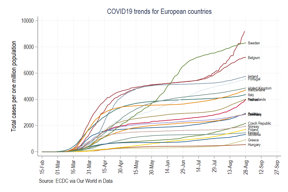
This guide will cover an important, yet, under-explored part of Stata: the use of custom color schemes. In summary, we will learn how to go from this graph:

本指南將涵蓋Stata的一個重要但尚未充分研究的部分：自定義配色方案的使用。 總而言之，我們將學習如何從該圖開始：

to this graph which implements a matplotlib color scheme, typically used in R and Python graphs, in Stata:

該圖實現了matplotlib配色方案 ，通常在Stata中用于R和Python圖：

This guide also touches upon advanced use of locals and loops which are essential for automation of tasks in Stata. Therefore, the guide assumes a basic knowledge of Stata commands. Understanding the underlying underlying logic here can also be applied to various Stata routines beyond generating graphs.

本指南還涉及高級使用局部變量和循環，這對于Stata中的任務自動化至關重要。 因此，本指南假定您具有Stata命令的基本知識。 除了生成圖形外，了解此處的基本邏輯還可以應用于各種Stata例程。

This guide build on the first article where data management, folder structures, and an introduction to automation of tasks are discussed in detail. While it is highly recommended to follow the first guide to set up the data and the folders, for the sake of completeness, some basic information is repeated here.

本指南以第一篇文章為基礎 ，其中詳細討論了數據管理，文件夾結構以及任務自動化的簡介。 雖然強烈建議您遵循第一本指南來設置數據和文件夾，但是為了完整起見，此處重復一些基本信息。

The guide follows a specific folder structure, in order to track changes in files. This folder structure and code used in the first guide can be downloaded from Github.

該指南遵循特定的文件夾結構，以便跟蹤文件中的更改。 可以從Github下載此第一指南中使用的文件夾結構和代碼。

In case you are starting from scratch, create a main folder and the following five sub-folders within the root folder:

如果您是從頭開始，請在根文件夾中創建一個主文件夾和以下五個子文件夾：

This will allow you to use the code, that makes use of relative paths, given in this guide.

這將允許您使用本指南中提供的使用相對路徑的代碼。

The guide is split into five steps:

該指南分為五個步驟：

• Step 1: provides a quick summary on setting up the COVID-19 dataset from Our World in Data.

  第1步 ：提供有關從Our World in Data中建立COVID-19數據集的快速摘要。

• Step 2: discusses custom graph schemes for cleaning up the layout

  步驟2 ：討論用于清理布局的自定義圖形方案

• Step 3: introduces line graphs and their various elements

  步驟3 ：介紹折線圖及其各種元素

• Step 4: introduces color palettes and how to integrate them into line graphs

  第4步 ：介紹調色板以及如何將它們集成到折線圖中

• Step 5: shows how the whole process of generating graphs with custom color schemes can be automated using loops and locals

  步驟5 ：展示如何使用循環和局部變量自動生成帶有自定義配色方案的圖形的整個過程

步驟1：重新整理資料 (Step 1: A refresher on the data)

In case you are starting from scratch, start a new dofile, and set up the data using the following commands:

如果您是從頭開始的，請啟動一個新的文件，然后使用以下命令設置數據：

clear
cd <your main directory here with sub-folders shown above>***********************************
**** our worldindata ECDC dataset
***********************************insheet using "https://covid.ourworldindata.org/data/ecdc/full_data.csv", clear
save ./raw/full_data_raw.dta, replacegen year  = substr(date,1,4)
gen month = substr(date,6,2)
gen day   = substr(date,9,2)destring year month day, replace
drop date
gen date = mdy(month,day,year)
format date %tdDD-Mon-yyyy
drop year month day
gen date2 = date
order date date2drop if date2 < 21915gen group = .replace group = 1 if ///
 location == "Austria"         | /// 
 location == "Belgium"         | ///
 location == "Czech Republic"  | ///
 location == "Denmark"         | ///
 location == "Finland"         | ///
 location == "France"          | ///
 location == "Germany"         | ///
 location == "Greece"          | ///
 location == "Hungary"         | ///
 location == "Italy"           | ///
 location == "Ireland"         | ///
 location == "Netherlands"     | ///
 location == "Norway"          | ///
 location == "Poland"          | ///
 location == "Portugal"        | ///
 location == "Slovenia"        | ///
 location == "Slovak Republic" | ///
 location == "Spain"           | ///
 location == "Sweden"          | ///
 location == "Switzerland"     | ///
 location == "United Kingdom"keep if group==1ren location country
tab country
compress
save "./temp/OWID_data.dta", replace**** adding the population datainsheet using "https://covid.ourworldindata.org/data/ecdc/locations.csv", clear
drop countriesandterritories population_year
ren location country
compress
save "./temp/OWID_pop.dta", replace**** merging the two datasetsuse ./temp/OWID_data, clear
merge m:1 country using ./temp/OWID_popdrop if _m!=3
drop _m***** generating population normalized variablesgen total_cases_pop  = (total_cases  / population) * 1000000
gen total_deaths_pop = (total_deaths / population) * 1000000
***** clean up the datedrop if date < 21960
format date %tdDD-Mon
summ date***** identify the last date
summ date
gen tick = 1 if date == `r(max)'
***** save the file
compress
save ./master/COVID_data.dta, replace

步驟2：自定義圖形方案 (Step 2: Custom graph schemes)

In the first guide, we learnt how to make line graphs using the Stata’s xtline command. This was done by declaring the data to be a panel dataset. To summarize, we use the following commands to generate a panel data line graph:

在第一個指南中 ，我們學習了如何使用Stata的xtline命令制作線圖。 這是通過將數據聲明為面板數據集來完成的。 總而言之，我們使用以下命令來生成面板數據折線圖：

summ date
local start = `r(min)'
local end   = `r(max)' + 30xtline total_cases_pop ///
 , overlay ///
  addplot((scatter total_cases_pop date if tick==1, mcolor(black) msymbol(point) mlabel(country) mlabsize(vsmall) mlabcolor(black))) ///
  ttitle("") ///
  tlabel(`start'(15)`end', labsize(small) angle(vertical) grid) ///
  title(COVID19 trends for European countries) ///
  note(Source: ECDC via Our World in Data) ///
  legend(off) ///
  graphregion(fcolor(white)) ///
  scheme(s2color)
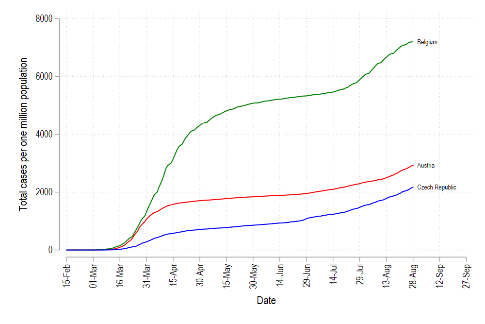
graph export ./graphs/medium2_graph1.png, replace wid(1000)

which gives us this figure:

這給了我們這個數字：

This figure uses the default color s2 color scheme in Stata where we manually adjusted the background colors, axes, labels, and headings. The font is set to Arial Narrow. In the code above, we add an additional feature to the graph code, scheme(s2color) to manually define which scheme we want to use.

此圖使用Stata中的默認顏色s2配色方案，在該方案中我們手動調整了背景色，軸，標簽和標題。 字體設置為Arial Narrow。 在上面的代碼中，我們在圖形代碼中添加了一個額外的功能Scheme(s2color)，以手動定義我們要使用的方案。

Rather than customizing minor elements of graphs ourselves, we can also rely on several user-written graph schemes. Stata does not have a central repository of these files, hence the files are scattered all over the internet. Here are are codes for accessing some clean colors schemes:

除了自己定制圖的次要元素外，我們還可以依靠幾種用戶編寫的圖方案。 Stata沒有這些文件的中央存儲庫，因此文件分散在整個Internet上。 以下是用于訪問一些干凈顏色方案的代碼：

net install scheme-modern, from("https://raw.githubusercontent.com/mdroste/stata-scheme-modern/master/")
summ date
local start = `r(min)'
local end   = `r(max)' + 30xtline total_cases_pop ///
 , overlay ///
  addplot((scatter total_cases_pop date if tick==1, mcolor(black) msymbol(point) mlabel(country) mlabsize(vsmall) mlabcolor(black))) ///
  ttitle("") ///
  tlabel(`start'(15)`end', labsize(small) angle(vertical)) ///
  title(COVID19 trends for European countries) ///
  note(Source: ECDC via Our World in Data) ///
  legend(off) ///
  scheme(modern)graph export ./graphs/medium2_graph2.png, replace wid(1000)

The modern scheme cleans up the background and the grids. So we do not have to add additional command lines like graphregion(fcolor(white)) and grid in the tlabel command since they are defined within the scheme.

現代方案可以清理背景和網格。 因此，我們不必在tlabel命令中添加諸如graphregion(fcolor(white))和grid之類的其他命令行，因為它們是在方案中定義的。

Tip: One can generate their own color schemes by following the official guide here.

提示：可以按照此處的官方指南來生成自己的配色方案。

The code above gives, us the following graph:

上面的代碼為我們提供了下圖：

Another popular scheme is cleanplots:

另一個流行的方案是cleanplots：

net install cleanplots, from("https://tdmize.github.io/data/cleanplots")summ date
local start = `r(min)'
local end   = `r(max)' + 30xtline total_cases_pop ///
 , overlay ///
  addplot((scatter total_cases_pop date if tick==1, mcolor(black) msymbol(point) mlabel(country) mlabsize(vsmall) mlabcolor(black))) ///
  ttitle("") ///
  tlabel(`start'(15)`end', labsize(small) angle(vertical) grid) ///
  title(COVID19 trends for European countries) ///
  note(Source: ECDC via Our World in Data) ///
  legend(off) ///
  scheme(cleanplots)  
graph export ./graphs/medium2_graph3.png, replace wid(1000)

Which modifies the line colors and the axis lines as well:

它也可以修改線條顏色和軸線：

This is the default scheme I use myself personally for all Stata graphs. One can also set the scheme permanently by typing the following command:

這是我個人用于所有Stata圖的默認方案。 也可以通過鍵入以下命令來永久設置方案：

set scheme cleanplots, perm

This tells Stata to replace the default s2 color scheme with cleanplots permanently.

這告訴Stata用cleanplots永久替換默認的s2配色方案。

步驟3：返回基本折線圖 (Step 3: Going back to the basic line graphs)

In this section, we will drop the xtline, panel graph command and go back to the very basic line graphs. The line graphs provide us with the building blocks to start customizing figures.

在本節中，我們將刪除xtline面板圖命令，然后返回最基本的線圖。 折線圖為我們提供了開始定制圖形的基礎。

The default line graph menu can be accessed from the interface as follows:

可以從界面訪問默認的折線圖菜單，如下所示：

and just click on the very first option:

只需單擊第一個選項：

and in the if tab, set the line graph to only show the country with id = 1 (Note the use of double == sign in the command).

然后在if標簽中，將折線圖設置為僅顯示id = 1的國家/地區(請注意在命令中使用double ==符號)。

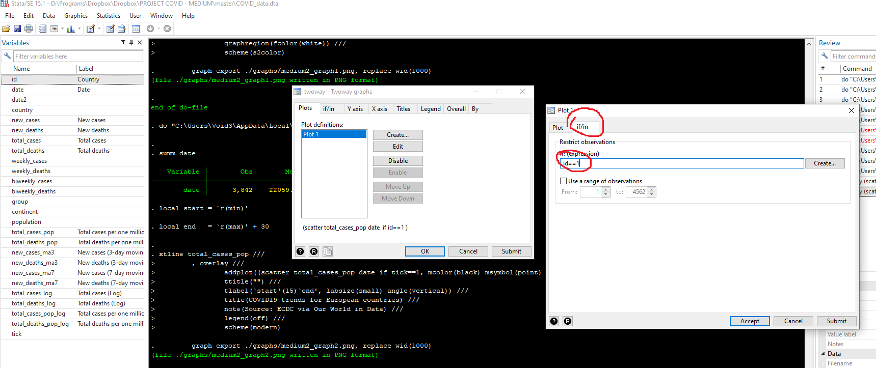
If you press submit, you will get the following syntax and graph:

如果按提交，您將獲得以下語法和圖形：

twoway ///
 (line total_cases_pop date if id==1) ///
 , legend(off)
 graph export ./graphs/medium2_graph5.png, replace wid(1000)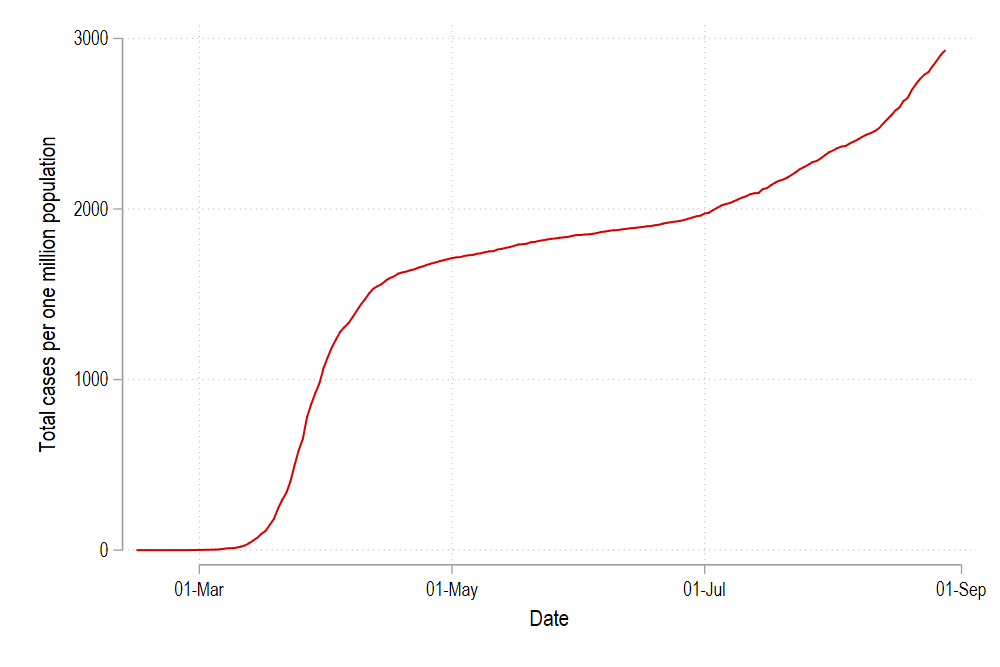

Which gives us just one line in the cleanplots color scheme for the country with id = 1. We can modify this line by changing the color and the line pattern simply by typing:

這給我們提供了id = 1的國家的cleanplots配色方案中的一行。我們可以通過簡單地鍵入以下內容來更改顏色和線條圖案來修改該線條：

twoway ///
 (line total_cases_pop date if id==1, lcolor(green) lpattern(dash)) ///
 , legend(off)graph export ./graphs/medium2_graph6.png, replace wid(1000)

or we can abbreviate the syntax a bit (where lc = line color, and lp = line pattern, and lw = line width):

或者我們可以稍微簡化一下語法(其中lc =線條顏色， lp =線條圖案， lw =線條寬度)：

twoway ///
 (line total_cases_pop date if id==1, lc(green) lp(solid)) ///
 , legend(off) 
 graph export ./graphs/medium2_graph7.png, replace wid(1000)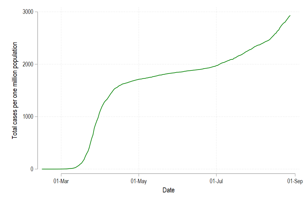

We can add more lines as well by modifying the code above and give the new lines green, blue, and red colors:

我們還可以通過修改上面的代碼來添加更多行，并將新行賦予綠色，藍色和紅色：

twoway ///
 (line total_cases_pop date if id==1, lc(green) lp(solid)) ///
 (line total_cases_pop date if id==2, lc(blue) lp(solid)) ///
 (line total_cases_pop date if id==3, lc(red) lp(solid)) ///
 , legend(off) 
 graph export ./graphs/medium2_graph8.png, replace wid(1000)

And we can add additional elements to neatly label this graph:

我們可以添加其他元素來整齊地標記此圖：

summ date
local start = `r(min)'
local end   = `r(max)' + 30twoway ///
 (line total_cases_pop date if id==1, lc(green) lp(solid)) ///
 (line total_cases_pop date if id==2, lc(blue) lp(solid)) ///
 (line total_cases_pop date if id==3, lc(red) lp(solid)) ///
 (scatter total_cases_pop date if tick==1 & id <= 3, mcolor(black) msymbol(point) mlabel(country) mlabsize(vsmall) mlabcolor(black)) ///
 , ///
  xlabel(`start'(15)`end', labsize(small) angle(vertical)) ///
  legend(off)
 graph export ./graphs/medium2_graph9.png, replace wid(1000)

In Stata colors can also be defined using RGB values. So for the graph above, the corresponding RGB values for the three graphs:

在Stata中，還可以使用RGB值定義顏色。 因此，對于上面的圖形，三個圖形的相應RGB值：

Red = “255 0 0”

紅色=“ 255 0 0”

Green = “0 128 0”

綠色=“ 0 128 0”

Blue = “0 0 255”

藍色=“ 0 0 255”

summ date
local start = `r(min)'
local end   = `r(max)' + 30twoway ///
 (line total_cases_pop date if id==1, lc("255 0 0") lp(solid)) ///
 (line total_cases_pop date if id==2, lc("0 128 0") lp(solid)) ///
 (line total_cases_pop date if id==3, lc("0 0 255") lp(solid)) ///
 (scatter total_cases_pop date if tick==1 & id <= 3, mcolor(black) msymbol(point) mlabel(country) mlabsize(vsmall) mlabcolor(black)) ///
 , ///
  xlabel(`start'(15)`end', labsize(small) angle(vertical)) ///
  legend(off)
 graph export ./graphs/medium2_graph10.png, replace wid(1000)

which gives us exactly the same graph as above:

這給了我們與上面完全相同的圖：

We can keep adding new lines and new colors as well, but this quickly becomes inefficient especially if we have a lot of countries. Manually defining a color for each line requires a lot of copy pasting and defining colors for each line.

我們也可以不斷添加新的線條和新的顏色，但是這很快變得效率低下，尤其是在我們有很多國家的情況下。 手動為每行定義顏色需要大量復制粘貼并為每行定義顏色。

In order to proceed further, we will work on two new elements:

為了進一步進行，我們將研究兩個新元素：

• Using color palettes to replace colors for individual lines
  使用調色板替換單個線條的顏色
• Generating loops to generate lines for all countries
  生成循環以生成所有國家/地區的線路

步驟4：使用調色板 (Step 4: Using color palettes)

Here we install two packages written by Benn Jann called palettes and colrspace:

以書面形式在這里，我們安裝兩個包鴨舌Jann稱為調色板和colrspace：

ssc install palettes, replace    // for color palettes
ssc install colrspace, replace   // for expanding the color base

One can also directly install from Github to make sure we have the very latest update:

也可以從Github直接安裝以確保我們具有最新更新：

net install palettes, replace from("https://raw.githubusercontent.com/benjann/palettes/master/")
net install colrspace, replace from("https://raw.githubusercontent.com/benjann/colrspace/master/")

The documentation of these packages can be checked here and one can also explore them by typing:

這些軟件包的文檔可以在此處檢查，也可以通過鍵入以下內容進行探索：

help colorpalette
help colrspace

Here we will not go into detail of the color theory, or the use of colors since this requires a whole guide on its own. But we will make use of the set of color schemes that come bundled with these packages. For example, colorpalette introduces the popular matplotlib color scheme typically used in R and Python graphs:

在這里，我們將不詳細介紹顏色理論或顏色的使用，因為這需要單獨的完整指南。 但是，我們將利用這些軟件包隨附的一組配色方案。 例如，colorpalette引入了流行的matplotlib配色方案，通常在R和Python圖形中使用：

colorpalette plasma
colorpalette inferno
colorpalette cividis
colorpalette viridis

The viridis color scheme can be easily recognized since it is one of the most used schemes in Python and R (e.g. in ggplots2). We can also generate different color ranges:

翠綠配色方案很容易識別，因為它是Python和R中最常用的配色方案之一(例如ggplots2)。 我們還可以生成不同的顏色范圍：

colorpalette viridis, n(10)
colorpalette: viridis, n(5) / viridis, n(10) / viridis, n(15)

where the last command gives us:

最后一條命令給我們的位置：

Here we can give whatever value of n to generate a linearly interpolated colors. In the next step, we incorporate the viridis color scheme in the 3 line graph we generate above:

在這里，我們可以給出n的任何值來生成線性插值的顏色。 下一步，我們將viridis配色方案合并到上面生成的3條線圖中：

colorpalette viridis, n(3) nograph    // 3 colors and no graph
return list                          // return the locals stored

The Stata window will show the following output. The key locals for us are r(p1), r(p2), r(p3), which contains the RGB code for the three colors we need to modify the graph. Now rather than copy pasting the RGB code, we can simply store this information in a set of locals:

Stata窗口將顯示以下輸出。 我們的主要局部變量是r(p1) ， r(p2) ， r(p3) ，其中包含我們需要修改圖形的三種顏色的RGB代碼。 現在，我們無需復制粘貼RGB代碼，而只需將這些信息存儲在一組本地語言中：

colorpalette viridis, n(3) nograph 
return listlocal color1 = r(p1)
local color2 = r(p2)
local color3 = r(p3)summ date
local start = r(min)
local end   = r(max) + 30twoway ///
 (line total_cases_pop date if id==1, lc("`color1'") lp(solid)) ///
 (line total_cases_pop date if id==2, lc("`color2'") lp(solid)) ///
 (line total_cases_pop date if id==3, lc("`color3'") lp(solid)) ///
 (scatter total_cases_pop date if tick==1 & id <= 3, mcolor(black) msymbol(point) mlabel(country) mlabsize(vsmall) mlabcolor(black)) ///
 , ///
  xlabel(`start'(15)`end', labsize(small) angle(vertical)) ///
  legend(off)
 graph export ./graphs/medium2_graph11.png, replace wid(1000)

which gives us this graph:

這給了我們這張圖：

and if we are using five countries:

如果我們使用五個國家：

colorpalette viridis, n(5) nograph  
return list
local color1 = r(p1)
local color2 = r(p2)
local color3 = r(p3)
local color4 = r(p4)
local color5 = r(p5)summ date
local start = r(min)
local end   = r(max) + 30twoway ///
 (line total_cases_pop date if id==1, lc("`color1'") lp(solid)) ///
 (line total_cases_pop date if id==2, lc("`color2'") lp(solid)) ///
 (line total_cases_pop date if id==3, lc("`color3'") lp(solid)) ///
 (line total_cases_pop date if id==4, lc("`color4'") lp(solid)) ///
 (line total_cases_pop date if id==5, lc("`color5'") lp(solid)) ///
 (scatter total_cases_pop date if tick==1 & id <= 5, mcolor(black) msymbol(point) mlabel(country) mlabsize(vsmall) mlabcolor(black)) ///
 , ///
  xlabel(`start'(15)`end', labsize(small) angle(vertical)) ///
  legend(off)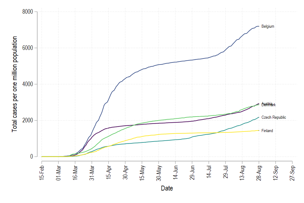

But here we see one problem: the color order is messed up. In order to fix the color graduation, we need to create a rank of countries from lowest to highest values (or vice versa) on the last date (which we have also marked with the variable tick). This can be done in Stata using the egen command:

但是在這里我們看到一個問題：顏色順序混亂了。 為了修正顏色分級，我們需要在最后一個日期(也用變量tick標記)上創建從最低值到最高值(反之亦然)的國家/地區等級。 這可以使用egen命令在Stata中完成：

egen rank = rank(total_cases_pop) if tick==1, f

Tip: See help egen for a complete list of very useful commands. Also check egenmore which extends the functionality of egen.

提示：有關非常有用的命令的完整列表，請參見help egen 。 還要檢查egenmore ，它擴展了egen的功能。

We can see that the correct order has been identified by typing:

我們可以看到通過鍵入以下命令確定了正確的訂單：

sort date rank 
br country date total_cases_pop rank if tick==1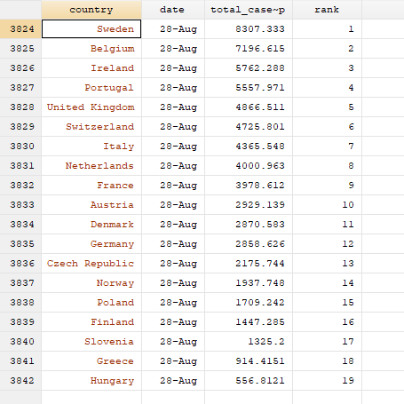

Here we can see that Sweden has the highest cumulative cases per million population and is ranked 1, while Hungary has the lowest cumulative cases per mission population and has a rank of 19.

在這里我們可以看到，瑞典每百萬人口的累積病例數最高，排名第1，而匈牙利每特派團人口的累積病例數最低，排名第19。

Now to get the correct colors, this ranking has to be applied to ALL the past observations as well. Here we introduce a level loop:

現在要獲得正確的顏色，此排名也必須應用于所有過去的觀察結果。 在這里，我們介紹一個級別循環：

levelsof country, local(lvls)
foreach x of local lvls {
 display "`x'"
 qui summ rank if country=="`x'"  // summarize the rank of country x
 cap replace rank = `r(max)' if country=="`x'" & rank==.
 }

Tip: Levels of individual unique elements within a variable. The levelsof command help automating looping over all unique values without having to manually define them.

提示：變量中各個唯一元素的級別。 levelof命令可幫助自動循環所有唯一值，而無需手動定義它們。

The first command levelsof, stores all the unique values of countries in the local lvls. foreach loops over each lvl (see help forheach). The command display shows the country we are currently looping. qui stands for quietly, and it hides displaying the summarize (summ) command in the Stata output window. This is strictly not necessary. replace replaces the rank variable with the max value returned from the summarize command above for each country and for all empty observations. The capture command (cap), effectively skips the execution of this command if an error occurs. This is a powerful command that allows us to bypass code errors. Errors stop the executing of the code and display an error. capture should only be used if you know exactly what you are doing. The reason we use it here, is because one country (Spain) does not have an observation for the last date. Hence the summarize command returns nothing and therefore there is nothing to be replaced. We can fine tune this code, but this requires adding additional elements not necessary for this guide. We will leave it for other guides in the future.

第一個命令levelof ，將國家的所有唯一值存儲在本地lvls中 。 foreach在每個lvl上循環(請參閱help forheach) 。 命令顯示將顯示我們當前正在循環播放的國家/地區。 qui安靜地代表，它隱藏在Stata輸出窗口中顯示summary ( summ )命令。 完全沒有必要。 replace將上述變量替換為上面的summary命令為每個國家和所有空觀測值返回的最大值的等級變量。 如果發生錯誤，那么捕獲命令( cap )有效地跳過該命令的執行。 這是一個功能強大的命令，可讓我們繞過代碼錯誤。 錯誤會停止執行代碼并顯示錯誤。 僅當您確切知道自己在做什么時，才應使用捕獲 。 我們在這里使用它的原因是因為一個國家(西班牙)沒有最后日期的觀測值。 因此，summary命令不返回任何內容，因此沒有任何要替換的內容。 我們可以對此代碼進行微調，但這需要添加本指南中不必要的其他元素。 將來我們會將其留給其他指南使用。

Once the ranks are defined, we now generate the graph again, BUT, this time we do not plot on the variable id, but on the variable rank:

定義等級后，我們現在再次生成圖形，但這次，我們不會在變量id上繪制，而是在變量等級上繪制：

colorpalette viridis, n(5) nograph  
return list
local color1 = r(p1)
local color2 = r(p2)
local color3 = r(p3)
local color4 = r(p4)
local color5 = r(p5)summ date
local start = r(min)
local end   = r(max) + 30twoway ///
 (line total_cases_pop date if rank==1, lc("`color1'") lp(solid)) ///
 (line total_cases_pop date if rank==2, lc("`color2'") lp(solid)) ///
 (line total_cases_pop date if rank==3, lc("`color3'") lp(solid)) ///
 (line total_cases_pop date if rank==4, lc("`color4'") lp(solid)) ///
 (line total_cases_pop date if rank==5, lc("`color5'") lp(solid)) ///
 (scatter total_cases_pop date if tick==1 & rank <= 5, mcolor(black) msymbol(point) mlabel(country) mlabsize(vsmall) mlabcolor(black)) ///
 , ///
  xlabel(`start'(15)`end', labsize(small) angle(vertical)) ///
  legend(off) 
 graph export ./graphs/medium2_graph13.png, replace wid(1000)

which gives us:

這給了我們：

Since the variables id and rank are not the same, we get a different set of countries. But the main thing here is that all lines are colored in the correct order.

由于變量id和rank不相同，因此我們得到了一組不同的國家。 但是這里最主要的是所有行都按正確的順序著色。

步驟5：全自動 (Step 5: Full automation)

Now we come to trickiest part of the code: adding all the countries and generating their corresponding colors. Here the code will get fairly complex, but we will go over the logic step-by-step.

現在我們來看代碼中最棘手的部分：添加所有國家/地區并生成其相應的顏色。 這里的代碼將變得相當復雜，但我們將逐步講解邏輯。

First, lines cannot be added manually for each country. Especially if we are using different country groupings with different number of countries. Stata, by default, has no option of batch modifying lines in graphs. This is probably only possible in the panel data, xtline command but it also has limited functionality when it comes to modifying the elements of each line. In order to bypass this limitation, what we can do is generate the graph command using locals and loops. If we look at the graph commands above, there is a pattern to how the lines are generated:

首先，不能為每個國家/地區手動添加行。 尤其是當我們使用不同國家/地區的不同國家/地區分組時。 默認情況下，Stata不能批量修改圖形中的線。 這可能僅在面板數據xtline命令中可行，但在修改每行的元素時功能也有限。 為了繞過此限制，我們可以做的是使用局部變量和循環生成graph命令。 如果我們看一下上面的graph命令，將有一條直線生成方式：

(line total_cases_pop date if rank==1, lc("`color1'") lp(solid)) ///
(line total_cases_pop date if rank==2, lc("`color2'") lp(solid)) ///

First line says rank = 1 and lc(..color1..), second line says rank=2 and color2 etc. Thus the numbers define both the rank and the color value. Hence, if we know the total number of countries, we can loop over them and sequentially generate code for each line.

第一行表示等級= 1和lc(.. color1 ..)，第二行表示等級= 2和color2等。因此，數字定義了等級和顏色值。 因此，如果我們知道國家/地區的總數，則可以遍歷國家/地區并為每一行依次生成代碼。

Since this is a non-standard Stata graph procedure, I will give the code for looping over the total observations and generating these lines:

由于這是一個非標準的Stata圖過程，因此我將給出用于遍歷總觀測值并生成以下行的代碼：

levelsof rank, local(lvls)   // loop over all the levels
local items = r(r)           // pick the total items foreach x of local lvls {
 colorpalette viridis, n(`items') nograph local customline `customline' (line total_cases_pop date if rank == `x', lc("`r(p`x')'") lp(solid)) ||
  }

and discuss it here:

并在這里討論：

levelsof generates the unique values of rank, which also equals the number of countries (each country has a unique rank). local items store the total number of unique rank values for use later. foreach loops over all the rank levels. For each level, a colorpalette for the viridis color scheme is generated for the number of countries defined in the local items.

levelof生成唯一的等級值，也等于國家/地區的數量(每個國家/地區都有唯一的等級)。 本地項目存儲唯一等級值的總數，以供以后使用。 foreach在所有等級上循環。 對于每個級別，將針對本地項目中定義的國家/地區數量生成viridis配色方案的調色板 。

The next command stores the information for each rank in local called customline. Every time the loop goes on to the next rank value, the information of the new line graph is appended to the existing line. Each line is given a color value r(px), where x is the rank order and r(px) is the corresponding color value from the colorpalette for that specific rank.

下一條命令將每個等級的信息存儲在本地稱為customline的行中。 每當循環繼續到下一個等級值時，新折線圖的信息就會附加到現有折線上。 每行都有一個顏色值r(p x )，其中x是等級順序，r(p x )是該特定等級的調色板中對應的顏色值。

Note that this type of programming is fairly common in softwares like Matlab, Mathematica, and R as well which mostly work with lists and matrices.

請注意，這種類型的編程在Matlab，Mathematica和R等軟件中也很常見，這些軟件主要用于列表和矩陣。

The double pipe command (||), is Stata’s internal command for splitting line graphs. Essentially the local customline contains information on all the lines for all the countries. This can be used as follows:

雙管道命令(||)是Stata的內部折線圖命令。 本質上，本地定制行包含有關所有國家/地區的所有行的信息。 可以如下使用：

levelsof rank, local(lvls)   // loop over all the levels
local items = r(r)foreach x of local lvls {
 colorpalette viridis, n(`items') nographlocal customline `customline' (line total_cases_pop date if rank == `x', lc("`r(p`x')'") lp(solid)) ||
  }summ date
local start = r(min)
local end   = r(max) + 30twoway `customline' ///
 (scatter total_cases_pop date if tick==1 & rank <= `items', mcolor(black) msymbol(point) mlabel(country) mlabsize(vsmall) mlabcolor(black)) ///
 , ///
  xlabel(`start'(15)`end', labsize(small) angle(vertical)) ///
  xtitle("") ///
  title("COVID-19 trends for European countries") ///
  note("Source: ECDC via Our World in Data", size(vsmall)) ///
  legend(off) 
graph export ./graphs/medium2_graph_final.png, replace wid(1000)

Which gives us this neat looking graph:

這給了我們這個整潔的圖形：

The code above can be used with any number of lines to auto color and label the line graphs. This logic of loop and automation of code can also be used for any complex operation involving different groups and different level sizes.

上面的代碼可與任意數量的線一起使用，以自動為線圖著色和標記。 這種循環邏輯和代碼自動化也可以用于涉及不同組和不同級別大小的任何復雜操作。

行使 (Exercise)

Try generating the graph with different a country grouping and another color scheme.

嘗試使用其他國家/地區分組和另一種配色方案生成圖形。

其他指南 (Other guides)

Part 1: An introduction to data setup and customized graphs

第1部分：數據設置和自定義圖的介紹

Part 2: Customizing colors schemes

第2部分：自定義配色方案

Part 3: Heat plots

第3部分：熱圖

If you enjoy these guides and find them useful, then please like and follow my Medium Stata blog: <do> The Stata Guide

如果您喜歡這些指南并發現它們很有用，請喜歡并關注我的Medium Stata博客： <do> Stata指南

關于作者 (About the author)

I am an economist by profession and I have been using Stata for almost 18 years. I have worked and lived across three different continents. I am currently based in Vienna, Austria. You can find my research work on ResearchGate and codes repository on GitHub. You can follow my COVID-19 related Stata visualizations on my Twitter. I am also featured on the COVID19 Stata webpage in the visualization and graphics section.

我是一名經濟學家，并且已經使用Stata近18年了。 我曾在三個不同的大陸工作和生活過。 我目前居住在奧地利維也納。 您可以在ResearchGate和GitHub上的代碼存儲庫中找到我的研究工作。 您可以在Twitter上關注與COVID-19相關的Stata可視化。 我還出現在COVID19 Stata網頁的“可視化和圖形”部分中。

You can connect with me via Medium, Twitter, LinkedIn or simply through email: asjadnaqvi@gmail.com.

您可以通過Medium ， Twitter ， LinkedIn或通過電子郵件與我們聯系：asjadnaqvi@gmail.com。

My Medium blog for Stata stories here: <do> The Stata Guide

我的Stata故事我的中型博客： <do> Stata指南