In this post, I would like to invite you to continue our intuitive exploration of A/B testing, as seen in the previous post:

在本文中，我想邀請您繼續我們對A / B測試的直觀探索，如前一篇文章所示：

Resuming what we saw, we were able to prove through simulations and intuition that there was a relationship between Website Version and Signup since we were able to elaborate a test with a Statistical Power of 79% that allowed us to reject the hypothesis that states otherwise with 95% confidence. In other words, we proved that behavior as bias as ours was found randomly, only 1.6% of the time.

繼續觀察，我們可以通過模擬和直覺來證明網站版本和注冊之間存在關系，因為我們能夠以79％的統計功效精心制作一個測試，從而可以拒絕采用以下方法得出的假設： 95％的信心。 換句話說，我們證明了像我們這樣的偏見行為是隨機發現的，只有1.6％的時間。

Even though we were satisfied with the results, we still need to prove with a defined statistical confidence level that there was a higher-performing version. In practice, we need to prove our hypothesis that, on average, we should expect version F would win over any other version.

即使我們對結果感到滿意，我們仍然需要以定義的統計置信度證明存在更高性能的版本。 在實踐中，我們需要證明我們的假設，即平均而言，我們應該期望版本F會勝過任何其他版本。

開始之前 (Before we start)

Let us remember and explore our working data from our prior post, where we ended up having 8017 Dices thrown as defined by our Statistical Power target of 80%.

讓我們記住并探索我們先前職位的工作數據，最終我們拋出了8017個骰子，這是我們80％的統計功效目標所定義的。

# Biased Dice Rolling FunctionDiceRolling <- function(N) {
    Dices <- data.frame()
    for (i in 1:6) {
      if(i==6) {
        Observed <- data.frame(Version=as.character(LETTERS[i]),Signup=rbinom(N/6,1,0.2))
      } else {
        Observed <- data.frame(Version=as.character(LETTERS[i]),Signup=rbinom(N/6,1,0.16))
      }
      Dices <- rbind(Dices,Observed)
    }
    return(Dices)
}# In order to replicateset.seed(11)
Dices <- DiceRolling(8017) # We expect 80% Power
t(table(Dices))

As a reminder, we designed an R function that simulates a biased dice in which we have a 20% probability of lading in 6 while a 16% chance of landing in any other number.

提醒一下，我們設計了一個R函數，該函數可以模擬有偏見的骰子，在該骰子中，我們有20％的概率在6中提貨，而在其他數字中有16％的機會著陸。

Additionally, we ended up generating a dummy dataset of 8.017 samples, as calculated for 80% Power, that represented six different versions of a signup form and the number of leads we observed on each. For this dummy set to be random and have a winner version (F) that will serve us as ground truth, we generated this table by simulating some biased dice’s throws.

此外，我們最終生成了一個8017次冪計算的8.017個樣本的虛擬數據集，該數據集表示六個不同版本的注冊表單以及我們在每個表單上觀察到的潛在客戶數量。 為了使這個虛擬集是隨機的，并且有一個獲勝者版本(F)，它將用作我們的 基礎事實，我們通過模擬一些有偏向的骰子投擲來生成此表。

The output:

輸出：

Which should allow us to produce this report:

這應該使我們能夠生成此報告：

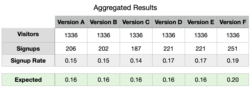
As seen above, we can observe different Signup Rates for our landing page versions. What is interesting about this is the fact that even though we planned a precise Signup Probability (Signup Rate), we got utterly different results between our observed and expected (planned) rates.

如上所述，對于目標網頁版本，我們可以觀察到不同的注冊率。 有趣的是，即使我們計劃了精確的注冊概率(注冊率)，我們在觀察到的和預期的(計劃的)利率之間卻得到了截然不同的結果。

Let us take a pause and allow us to conduct a “sanity check” of say, Version C, which shows the highest difference between its Observed (0.14) and Expected (0.16) rates in order to check if there is something wrong with our data.

讓我們暫停一下，讓我們進行一次“健全性檢查”，例如版本C，該版本顯示其觀測(0.14)和預期(0.16)速率之間的最大差異，以便檢查我們的數據是否存在問題。

完整性檢查 (Sanity Check)

Even though this step is not needed, it will serve us as a good starting point for building the intuition that will be useful for our primary goal.

即使不需要這一步驟，它也將為我們建立直覺提供一個很好的起點，這種直覺將對我們的主要目標有用。

As mentioned earlier, we want to prove that our results, even though initially different from what we expected, should not be far different from it since they vary based on the underlying probability distribution.

如前所述，我們想證明我們的結果，盡管最初與我們的預期有所不同，但應該與結果相差無幾，因為它們基于潛在的概率分布而變化。

In other words, for the particular case of Version C, our hypothesis are as follows:

換句話說，對于版本C的特定情況，我們的假設如下：

我們為什么使用手段？ (Why did we use means?)

This particular case allows us to use both proportions or means since, as we designed our variables to be dichotomous with values 0 or 1, the mean calculation represents, in this case, the same value as our ratios or proportions.

這種特殊的情況下，允許我們使用這兩個比例或辦法，因為正如我們在設計變量是二分與值0或1，平均值計算表示，在這種情況下，相同的值作為我們的比率或比例。

# Results for Version C
VersionC <- Dices[which(Dices$Version==”C”),]# Mean calculation
mean(VersionC$Signup)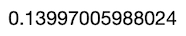

p值 (p-Value)

We need to find our p-Value, which will allow us to accept or reject our hypothesis based on the probability of finding results “as extreme” as the one we got for Version C within the underlying probability distribution.

我們需要找到我們的p值，這將使我們能夠基于在潛在概率分布內發現與版本C一樣“極端”的結果的概率來接受或拒絕我們的假設。

This determination, meaning that our mean is significantly different from a true value (0.16), is usually addressed through a variation of the well-known Student Test called “One-Sample t-Test.” Note: since we are also using proportions, we could also be using a “Proportion Test”, though it is not the purpose of this post.

這種確定意味著我們的平均值與真實值(0.16)顯著不同，通常通過一種著名的學生測驗(稱為“ 單樣本t測驗 ”)來解決。 注意：由于我們也使用比例，因此我們也可以使用“ 比例測試 ”，盡管這不是本文的目的。

To obtain the probability of finding results as extreme as ours, we would need to repeat our data collection process many times. Since this procedure is expensive and unrealistic, we will use a method similar to the resampling by permutation that we did in our last post called “Bootstrapping”.

為了獲得發現與我們一樣極端的結果的可能性，我們將需要重復多次數據收集過程。 由于此過程昂貴且不切實際，因此我們將使用類似于上一篇名為“ Bootstrapping”的文章中介紹的通過置換重采樣的方法。

自舉 (Bootstrapping)

Bootstrapping is done by reshuffling one of our columns, in this case Signups, while maintaining the other one fixed. What is different from the permutation resample we have done in the past is that we will allow replacement as shown below:

通過重新組合我們其中一列(在本例中為Signups)，同時保持另一列固定不變來進行引導。 與過去進行的排列重采樣不同的是，我們將允許替換，如下所示：

It is important to note that we need to allow replacement within this reshuffling process; otherwise, simple permutation will always result in the same mean as shown below.

重要的是要注意，我們需要允許在此改組過程中進行替換； 否則，簡單的置換將始終產生如下所示的均值。

Let us generate 10 Resamples without replacement:

讓我們生成10個重采樣而不替換 ：

i = 0
for (i in 1:10) {
 Resample <- sample(VersionC$Signup,replace=FALSE);
 cat(paste("Resample #",i," : ",mean(Resample),"\n",sep=""));
 i = i+1;
}

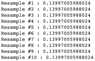
And 10 Resamples with replacement:

并替換 10個重采樣：

i = 0
for (i in 1:10) {
 Resample <- sample(VersionC$Signup,replace=TRUE);
 cat(paste("Resample #",i," : ",mean(Resample),"\n",sep=""));
 i = i+1;
}

模擬 (Simulation)

Let us simulate 30k permutations of Version C with our data.

讓我們用數據模擬版本C的30k排列。

# Let’s generate a Bootstrap and find our p-Value, Intervals and T-Scoresset.seed(1984)
Sample <- VersionC$Signup
score <- NULL
means <- NULL
for(i in 1:30000) {
 Bootstrap <- sample(Sample,replace = TRUE)
 means <- rbind(means,mean(Bootstrap))
 SimulationtTest <- tTest((Bootstrap-mean(Sample))/sd(Sample))
 tScores <- rbind(score,SimulationtTest)
}

As result, we got:

結果，我們得到：

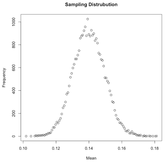
Initially, one might expect a distribution similar in shape, but centered around 0.16, therefore resembling the “true population mean” distribution. Even though we did not recreate the exact “ground truth distribution” (the one we designed), since it is now centered in the mean of our sample instead (0.14), we did recreate one that should have roughly the same shape and Standard Error, and that should contain within its range our true mean.

最初，人們可能會期望形狀相似的分布，但以0.16為中心，因此類似于“ 真實總體均值 ”分布。 即使我們沒有重新創建精確的“地面事實分布”(我們設計的)，因為它現在正以樣本均值(0.14)為中心，所以我們確實重新創建了形狀和標準誤差大致相同的模型，并且應該在其真實范圍內。

We can compare our “bootstrapped standard error” with the “true mean standard error” by using both Central Limit Theorem and the Standard Deviation formula for the Binomial Distribution.

通過使用中心極限定理和二項分布的標準偏差公式，我們可以將“ 自舉標準誤差 ”與“ 真實平均標準誤差 ”進行比較。

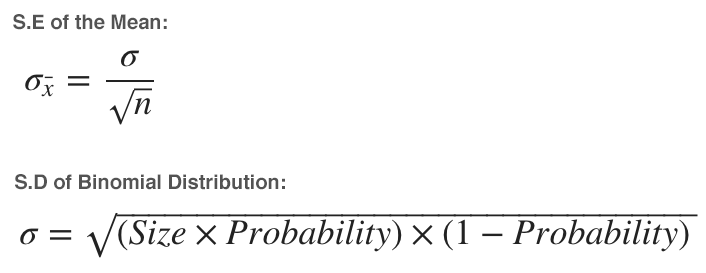
Which allow us to obtain:

這使我們可以獲得：

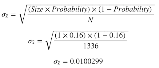
Which seems to be quite near to our bootstrapped Standard Error:

這似乎很接近我們自舉的標準錯誤：

# Mean from sampling distributionround(sd(means),6)

This data should be enough for us to approximate the original true mean distribution by simulating a Normal Distribution with a mean equal to 0.16 and a Standard Error of 0.01. We could find the percent of times a value as extreme as 0.14 is observed with this information.

通過模擬均值等于0.16且標準誤差為0.01的正態分布，該數據應該足以使我們近似原始的真實均值分布。 通過此信息，我們可以找到一個值達到0.14的極高次數的百分比。

As seen above, both our True Mean Distribution (green) and our Bootstrapped Sample Distribution (blue) seems very similar, except the latter is centered around 0.14.

如上所示，我們的真實均值分布(綠色)和自舉樣本分布(藍色)看起來非常相似，只是后者的中心在0.14左右。

At this point, we could solve our problem by either finding the percent of times a value as extreme as 0.14 is found within our true mean distribution (area colored in blue). Alternatively, we could find the percent of times a value as extreme as 0.16 is found within our bootstrapped sample distribution (area colored in green). We will proceed with the latter since this post is focused on simulations based solely on our sample data.

在這一點上，我們可以通過在真實的均值分布 (藍色區域)中 找到等于0.14的極值的次數百分比來解決問題。 或者，我們可以 在自舉樣本分布 (綠色區域)中 找到一個值達到0.16的極限值的百分比 。 我們將繼續進行后者，因為本文僅關注基于樣本數據的模擬。

Resuming, we need to calculate how many times we observed values as extreme as 0.16 within our bootstrapped sample distribution. It is important to note that in this case, we had a sample mean (0.14) inferior to our expected mean of 0.16, but that is not always the case since, as we saw in our results, Version D got 0.17.

繼續，我們需要計算在自舉樣本分布中觀察到的值高達0.16的次數。 重要的是要注意，在這種情況下，我們的樣本均值(0.14)低于我們的預期均值0.16，但并非總是如此，因為正如我們在結果中看到的，D版本的值為0.17。

In particular, we will perform a “two-tailed test”, which means finding the probability of obtaining values as extreme or as far from the mean as 0.16. Being our sample mean for Version C equal to 0.14, this is equivalent to say as low as 0.12 or as high as 0.16 since both values are equally extreme.

特別是，我們將執行“雙尾檢驗”，這意味著找到獲得的值作為極端 或 遠離平均0.16的概率。 作為我們對于版本C的樣本均值等于0.14，這等效于低至0.12或高至0.16，因為兩個值都同樣極端。

For this case, we found:

對于這種情況，我們發現：

# Expected Means, Upper and Lower interval (0.14 and 0.16)ExpectedMean <- 0.16
upper <- mean(means)+abs(mean(means)-ExpectedMean)
lower <- mean(means)-abs(mean(means)-ExpectedMean)
PValue <- mean(means <= lower | means >= upper)
Sum <- sum(means <= lower | means >= upper)
cat(paste(“We found values as extreme: “,PValue*100,”% (“,Sum,”/”,length(means),”) of the times”,sep=””))

Ok, we have found our p-Value, which is relatively low. Now we would like to find the 95% confidence interval of our mean, which would shed some light as of which values it might take considering a Type I Error (Alpha) of 5%.

好的，我們找到了相對較低的p值。 現在，我們想找到平均值的95％置信區間 ，這將為我們考慮5％的I型錯誤(Alpha)時取哪些值提供了一些啟示 。

# Data aggregation
freq <- as.data.frame(table(means))
freq$means <- as.numeric(as.character(freq$means))# Sort Ascending for right-most proportion
freq <- freq[order(freq$means,decreasing = FALSE),]
freq$cumsumAsc <- cumsum(freq$Freq)/sum(freq$Freq)
UpperMean <- min(freq$means[which(freq$cumsumAsc >= 0.975)])# Sort Descending for left-most proportion
freq <- freq[order(freq$means,decreasing = TRUE),]
freq$cumsumDesc <- cumsum(freq$Freq)/sum(freq$Freq)
LowerMean <- max(freq$means[which(freq$cumsumDesc >= 0.975)])# Print Results
cat(paste(“95 percent confidence interval:\n “,round(LowerMean,7),” “,round(UpperMean,7),sep=””))

Let us calculate our Student’s T-score, which is calculated as follows:

讓我們計算學生的T分數，其計算方法如下：

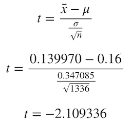
Since we already calculated this formula for every one of our 30k resamples, we can generate our critical t-Scores for 90%, 95%, and 99% confidence intervals.

由于我們已經為每30k次重采樣計算了此公式，因此我們可以生成90％，95％和99％置信區間的臨界t分數。

# Which are the T-Values expected for each Confidence level?
histogram <- data.frame(X=tScores)
library(dplyr)
histogram %>% 
 summarize(
 # Find the 0.9 quantile of diff_perm’s stat
 q.90 = quantile(X, p = 0.9),
 # … and the 0.95 quantile
 q.95 = quantile(X, p = 0.95),
 # … and the 0.99 quantile
 q.99 = quantile(X, p = 0.99)
 )

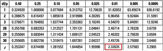
These values are very near the original Student’s Score Table for 1335 (N-1) degrees of freedom as seen here:

這些值非常接近原始學生的1335(N-1)自由度的成績表，如下所示：

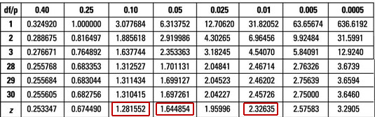
Resuming, we can observe that our calculated p-Value was around 3.69%, our 95% interval did not include 0.16, and our absolute t-Score of 2.1, as seen in our table, was just between the score of Alpha 0.05 and 0.01. All this seems to be coherent with the same outcome; we reject the null hypothesis with 95% confidence, meaning we cannot confirm that Version C’s true mean is equal to 0.16.

繼續，我們可以觀察到，我們計算出的p值約為3.69％，我們的95％區間不包括0.16，而我們的表中所見，我們的絕對t分數為2.1，正好在Alpha得分0.05和0.01之間。 所有這些似乎都與相同的結果相吻合。 我們以95％的置信度拒絕原假設 ，這意味著我們無法確認版本C的真實均值等于0.16。

We designed this test ourselves, and we know for sure our null hypothesis was correct. This concept of rejecting a true null hypothesis is called a False Positive or Type I Error, which can be avoided by increasing our current confidence Interval from 95% to maybe 99%.

我們自己設計了這個測試，并且我們肯定知道我們的零假設是正確的。 拒絕真實零假設的概念稱為誤報或I型錯誤，可以通過將當前的置信區間從95％增加到99％來避免。

So far, we have performed the equivalent of a “One-Sample t-Test” trough simulations, which implies we have determined whether the “sample mean” of 0.14 was statistically different from a known or hypothesized “population mean” of 0.16, which is our ground truth.

到目前為止，我們已經執行了與“ 單樣本t檢驗 ”低谷模擬等效的操作，這意味著我們已確定0.14的“樣本平均值”是否與已知或假設的0.16的“人口平均值”在統計上不同。是我們的基本真理。

For now, this will serve us as a building block for what is coming next since we will now proceed with a very similar approach to compare our Landing Versions between them to see if there is a winner.

目前，這將成為下一步工作的基礎，因為我們現在將采用一種非常相似的方法來比較它們之間的著陸版本，以查看是否有贏家。

尋找我們的贏家版本 (Finding our winner version)

We have explored how to compare if a Sample Mean was statistically different from a known Population Mean; now, let us compare our Sample Mean with another Sample Mean.

我們已經探索了如何比較樣本平均值是否與已知的總體平均值有統計學差異； 現在，讓我們將樣本均值與另一個樣本均值進行比較。

For this particular example, let us compare Version F vs. Version A.

對于此特定示例，讓我們比較版本F與版本A。

This procedure of comparing two independent samples is usually addressed with a test called “Unpaired Two sample t-Test”; it is unpaired since we will use different (independent) samples; we assume they behave randomly, with normal distribution and zero covariance, as we will later observe.

比較兩個獨立樣本的過程通常通過稱為“未配對的兩個樣本t檢驗”的測試解決 。 它是不成對的，因為我們將使用不同的(獨立的)樣本； 我們假設它們的行為隨機，正態分布且協方差為零，我們將在后面觀察到。

If we were to use the same sample, say at different moments in time, we would use a “Paired Two Sample t-Test” which, in contrast, compares two dependent samples, and it assumes a non-zero covariance which would be reflected in the formula.

如果我們使用相同的樣本，例如在不同的時刻，我們將使用“ 成對的兩個樣本t檢驗 ”，相比之下，它比較兩個相關樣本 ，并且假設將反映出一個非零協方差在公式。

In simple words, we want to know how often we observe a positive difference in means, which is equivalent to say that Version F has a higher mean than Version A, thus, better performance. We know our current difference in means is as follows:

用簡單的話說，我們想知道我們觀察到均值出現正差的頻率，這相當于說版本F的均值比版本A的均值高，因此性能更好。 我們知道我們目前的均值差異如下：

Since we know our Sample Means are just a single measurement of the real Population Mean for both Version F and Version A and not the true sample mean for neither one, we need to compute the estimated sample distribution for both versions like we did earlier. Unlike before, we will also calculate the difference in means for each resample to observe how it is distributed.

由于我們知道樣本均值僅是對版本F和版本A的真實總體均值的單次測量，而不是對兩個版本均不是真實的樣本均值 ，因此我們需要像之前所做的那樣計算兩個版本的估計樣本分布。 與以前不同，我們還將計算每次重采樣的均值差，以觀察其分布情況。

Let us simulate 40k samples with a replacement for Version F and Version A and calculate the difference in means:

讓我們模擬40k樣本，用版本F和版本A替代，并計算均值之差：

# Let’s select data from Version F and Version AVersionF <- Dices[which(Dices$Version==”F”),]
VersionA <- Dices[which(Dices$Version==”A”),]# We simulate 40kDiff <- NULL
meansA <- NULL
meansF <- NULL
for(i in 1:40000) {
 BootstrapA <- sample(VersionA$Signup,replace = TRUE)
 BootstrapF <- sample(VersionF$Signup,replace = TRUE)
 MeanDiff <- mean(BootstrapF)-mean(BootstrapA)
 Diff <- rbind(Diff,MeanDiff)
}# We plot the result
totals <- as.data.frame(table(Diff))
totals$Diff <- as.numeric(as.character(totals$Diff))
plot( totals$Freq ~ totals$Diff , ylab="Frequency", xlab="Difference",main="Sampling Difference Distrubution")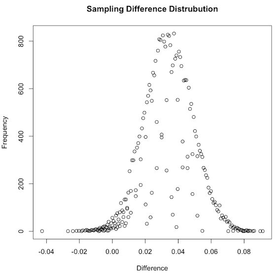

As we might expect from what we learned earlier, we got a normally distributed shape centered in our previously calculated sample difference of 0.337. Like before, we also know the difference between the true population means for Versions A and F should be within the range of this distribution.

正如我們可能從我們先前所學到的那樣，可以得到一個正態分布的形狀，其中心位于我們先前計算的樣本差異0.337中。 和以前一樣，我們也知道版本A和版本F 的真實總體均值之差應在此分布范圍內 。

Additionally, our bootstrap should have provided us a good approximation of the Standard Error of the difference between the true means. We can compare our “bootstrapped standard error” with the “true mean difference standard error” with both Central Limit Theorem and the Binomial Distribution.

此外，我們的自舉程序應該為我們提供了真實均值之差的標準誤差的良好近似值。 我們可以通過中心極限定理和二項分布來比較“ 自舉標準誤差 ”和“ 真實平均差標準誤差 ” 。

Which allow us to obtain:

這使我們可以獲得：

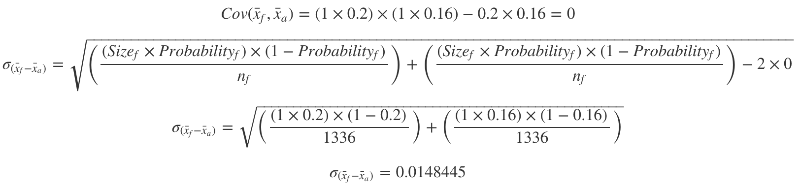
Just like before, it seems to be quite near our bootstrapped Standard Error for the difference of the means:

和以前一樣，由于方式的不同，這似乎已經很接近我們的標準錯誤了：

# Simulated Standard Error of the differencesround(sd(Diff),6)

As designed, we know the true expected difference of means is 0.04. We should have enough data to approximate a Normal Distribution with a mean equal to 0.04 and Standard Error of 0.0148, in which case we could find the percent of times a value as extreme as 0 is being found.

按照設計，我們知道均值的真實期望差是0.04。 我們應該有足夠的數據， 平均等于 正態分布逼近到 0.0148 0.04和標準錯誤，在這種情況下，我們能找到的時間百分比值極端的被發現0。

This scenario is unrealistic, though, since we would not usually have population means, which is the whole purpose of estimating trough confidence intervals.

但是，這種情況是不現實的，因為我們通常不會擁有總體均值，這是估計谷底置信區間的全部目的。

Contrary to our previous case, in our first example, we compared our sample distribution of Version C to a hypothesized population mean of 0.16. However, in this case, we compare two individual samples with no further information as it would happen in a real A/B testing.

與我們先前的情況相反，在我們的第一個示例中，我們將版本C的樣本分布與假設的總體平均值0.16進行了比較。 但是，在這種情況下，我們將比較兩個單獨的樣本，而沒有進一步的信息，因為這將在實際的A / B測試中發生。

In particular, we want to prove that Version F is superior to Version A, meaning that the difference between means is greater than zero. For this case, we need to perform a “One-Tailed” test answering the following question: which percent of the times did we observe a difference in means greater than zero?

特別是，我們要證明版本F優于版本A，這意味著均值之間的差大于零。 對于這種情況，我們需要執行“單尾”測試，回答以下問題： 在平均百分比中，觀察到差異大于零的百分比是多少？

Our hypothesis is as follows:

我們的假設如下：

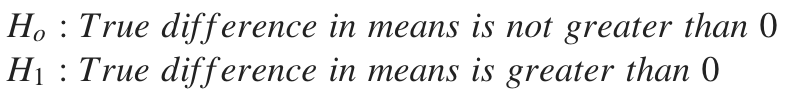
The answer:

答案：

# Percent of times greater than Zeromean(Diff > 0)

Since our p-Value represents the times we did not observe a difference in mean higher than Zero within our simulation, we can calculate it to be 0.011 (1–0.989). Additionally, being lower than 0.05 (Alpha), we can reject our null hypothesis; therefore, Version F had a higher performance than Version A.

由于我們的p值代表我們在仿真中未觀察到均值大于零的差異的時間，因此我們可以將其計算為0.011(1-0.989)。 此外，如果低于0.05(Alpha)，我們可以拒絕原假設 ； 因此，F 版本比A版本具有更高的性能。

If we calculate both 95% confidence intervals and t-Scores for this particular test, we should obtain similar results:

如果我們為此特定測試計算95％的置信區間和t分數，則我們應獲得類似的結果：

Confidence interval at 95%:

置信區間為95％：

# Data aggregation
freq <- as.data.frame(table(Diff))
freq$Diff <- as.numeric(as.character(freq$Diff))# Right-most proportion (Inf)UpperDiff <- Inf# Sort Descending for left-most proportion
freq <- freq[order(freq$Diff,decreasing = TRUE),]
freq$cumsumDesc <- cumsum(freq$Freq)/sum(freq$Freq)
LowerDiff <- max(freq$Diff[which(freq$cumsumDesc >= 0.95)])# Print Results
cat(paste(“95 percent confidence interval:\n “,round(LowerDiff,7),” “,round(UpperDiff,7),sep=””))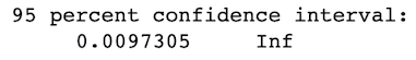

As expected, our confidence interval tells us that with 95% confidence, we should expect a difference of at least 0.0097, which is above zero; therefore, it shows a better performance.

不出所料，我們的置信區間告訴我們，在95％的置信度下，我們應該期望至少有0.0097的差異，該差異大于零。 因此，它表現出更好的性能。

Unpaired Two-Sample t-Test score:

未配對的兩次樣本t檢驗得分：

Similar to our previous values, checking our t-Table for T=2.31 and 2653 Degrees of Freedom we also found a p-Value of roughly 0.01

與我們之前的值類似，檢查t表中的T = 2.31和2653自由度，我們還發現p值大約為0.01

成對比較 (Pairwise Comparison)

So far, we have compared our Landing Page Version C with a hypothesized mean of 0.16. We have also compared Version F with Version A and found which was the highest-performer.

到目前為止，我們已經將目標網頁版本C與假設的平均值0.16進行了比較。 我們還將版本F和版本A進行了比較，發現性能最高。

Now we need to determine our absolute winner. We will do a Pairwise Comparison, meaning that we will test every page with each other until we determine our absolute winner if it exists.

現在我們需要確定我們的絕對贏家。 我們將進行成對比較，這意味著我們將相互測試每一頁，直到我們確定絕對贏家(如果存在)。

Since we will make a One-Tailed test for each and we do not need to test a version with itself, we can reduce the total number of tests as calculated below.

由于我們將為每個測試進行一次測試，因此我們不需要自己測試版本，因此可以減少如下計算的測試總數。

# Total number of versionsVersionNumber <- 6# Number of versions comparedComparedNumber <- 2# Combinationsfactorial(VersionNumber)/(factorial(ComparedNumber)*factorial(VersionNumber-ComparedNumber))

As output we obtain: 15 pair of tests.

作為輸出，我們獲得： 15對測試。

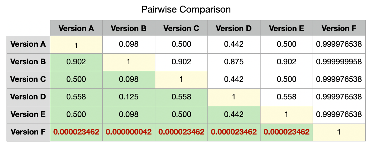
We will skip the process of repeating this 15 times, and we will jump straight to the results, which are:

我們將跳過重復此過程15次的過程，然后直接跳轉到以下結果：

As seen above, we have managed to find that Version F had better performance than both versions A, C, and was almost better performing than B, D, and E, which were close to our selected Alpha of 5%. In contrast, Version C seems to be an extraordinary case since, with both D and E, it seems to have a difference in means greater than zero, which we know is impossible since all three were designed with an equivalent probability of 0.16.

如上所示，我們設法發現版本F的性能優于版本A，C，并且幾乎比版本B，D和E更好，后者接近我們選擇的5％的Alpha。 相反，版本C似乎是一個特殊情況，因為對于D和E，它的均方差似乎都大于零，我們知道這是不可能的，因為所有這三個均以0.16的等效概率進行設計。

In other words, we have failed to reject our Null Hypothesis at a 95% confidence even though it is false for F vs. B, D, and C; this situation (Type II Error) could be solved by increasing our Statistical Power. In contrast, we rejected a true null hypothesis for D vs. C and E vs. C, which indicates we have incurred in a Type I Error, which could be solved by defining a lower Alpha or Higher Confidence level.

換句話說， 即使 F vs 是錯誤的 ，我們也無法以95％的置信度拒絕零假設 。 B， D和C; 這種情況(II型錯誤)可以通過提高統計功效來解決。 相反，我們拒絕了 D vs 的真實零假設 。 C和E 與 。 C，表示我們發生了I型錯誤 ，可以通過定義較低的Alpha或較高的置信度來解決。

We indeed designed our test to have an 80% statistical power. However, we designed it solely for testing differences between our total observed and expected frequencies and not for testing differences between individual means. In other words, we have switched from a “Chi-Squared Test” to an “Unpaired Two-Sample t-Test”.

實際上，我們將測試設計為具有80％的統計功效。 然而，我們設計它只是為了測試我們的 總 觀察和期望頻率 之間 ，而不是用于測試 個別 手段 之間的差異 的差異 。 換句話說，我們已經從“ 卡方檢驗”切換為““非配對兩樣本t檢驗””。

統計功效 (Statistical Power)

We have obtained our results. Even though we could use them as-is and select the ones with the highest overall differences, such as the ones with the lowest P-Values, we might want to re-test some of the variations in order to be entirely sure.

我們已經獲得了結果。 即使我們可以按原樣使用它們并選擇總體差異最大的差異(例如P值最低的差異)，我們也可能要重新測試某些差異以完全確定。

As we saw in our last post, Power is calculated as follows:

正如我們在上一篇文章中所見，Power的計算如下：

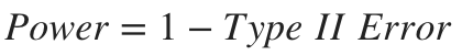
Similarly, Power is a function of:

同樣，Power是以下功能之一：

• Our significance criterion is our Type I Error or Alpha, which we decided to be 5% (95% confidence).

  我們的顯著性標準是I型錯誤或Alpha，我們決定為5％(置信度為95％)。

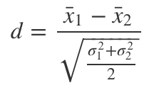
• Effect Magnitude or Size: This represents the difference between our observed and expected values regarding the standardized statistic of use. In this case, since we are using a Student’s Test Statistic, this effect (named d) is calculated as the “difference between means” divided by the “Pooled Standard Error”. It is usually categorized as Small (0.2), Medium (0.5), and Large (0.8).

  效果幅度或大小 ：這表示我們在有關標準化使用統計方面的觀察值與期望值之間的差異。 在這種情況下，由于我們使用的是學生的測試統計量，因此將這種效應(稱為d )計算為“ 均值之差”除以“ 合并標準誤差” 。 通常分為小(0.2)，中(0.5)和大(0.8)。

• Sample size: This represents the total amount of samples (in our case, 8017).

  樣本數量 ：代表樣本總數(在我們的情況下為8017)。

效果幅度 (Effect Magnitude)

We designed an experiment with a relatively small effect magnitude since our Dice was only biased in one face (6) with only a slight additional chance of landing in its favor.

我們設計的實驗的效果等級相對較小，因為我們的骰子僅偏向一張臉(6)，只有很少的其他機會落在其臉上。

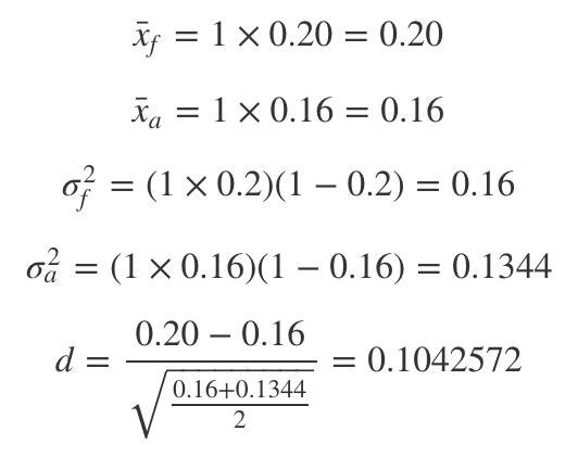
In simple words, our effect magnitude (d) is calculated as follows:

簡而言之，我們的影響幅度(d)計算如下：

If we calculate this for the expected values of Version F vs. Version A, using the formulas we have learned so far, we obtain:

如果我們使用到目前為止所學的公式針對版本F與版本A的期望值進行計算，則可以獲得：

樣本量 (Sample Size)

As we commented in our last post, we can expect an inverse relationship between sample sizes and effect magnitude. The more significant the effect, the lower the sample size needed to prove it at a given significance level.

正如我們在上一篇文章中評論的那樣，我們可以預期樣本量與效應量之間存在反比關系。 效果越顯著，在給定的顯著性水平下證明該結果所需的樣本量越少。

Let us try to find the sample size needed in order to have a 90% Power. We can solve this by iterating different values of N until we minimize the difference between our Expected Power and the Observed Power.

讓我們嘗試找到擁有90％功效的所需樣本量。 我們可以通過迭代N的不同值來解決此問題，直到我們將期望功率和觀察功率之間的差異最小化為止。

# Basic example on how to obtain a given N based on a target Power.
# Playing with initialization variables might be needed for different scenarios.
set.seed(11)
CostFunction <- function(n,d,p) {
  df <- (n - 1) * 2
  tScore <- qt(0.05, df, lower = FALSE)
  value <- pt(tScore , df, ncp = sqrt(n/2) * d, lower = FALSE)
  Error <- (p-value)^2
  return(Error)
}
SampleSize <- function(d,n,p) {
  # Initialize variables
  N <- n
  i <- 0
  h <- 0.000000001
  LearningRate <- 3000000
  HardStop <- 20000
  power <- 0
  # Iteration loop
  for (i in 1:HardStop) {
    dNdError <- (CostFunction(N + h,d,p) - CostFunction(N,d,p)) / h
    N <- N - dNdError*LearningRate
    tLimit <- qt(0.05, (N - 1) * 2, lower = FALSE)
    new_power <- pt(tLimit , (N- 1) * 2, ncp = sqrt(N/2) * d, lower = FALSE)
    if(round(power,6) >= p) {
      cat(paste0("Found in ",i," Iterations\n"))
      cat(paste0("   Power: ",round(power,2),"\n"))
      cat(paste0("   N: ",round(N)))
      break();
    }
    power <- new_power
    i <- i +1
  }
}
set.seed(22)
SampleSize((0.2-0.16)/sqrt((0.16+0.1344)/2),1336,0.9)

As seen above, after different iterations of N, we obtained a recommended sample of 1576 per dice to have a 0.9 Power.

如上所示，在N的不同迭代之后，我們獲得了每個骰子 1576的推薦樣本，具有0.9的功效。

Let us repeat the experiment from scratch and see which results we get for these new sample size of 9456 (1575*6) as suggested by aiming a good Statistical Power of 0.9.

讓我們從頭開始重復實驗，看看針對9456(1575 * 6)的這些新樣本大小，我們通過將0.9的良好統計功效作為目標而獲得了哪些結果。

# Repeat our experiment with sample size 9446set.seed(11)
Dices <- DiceRolling(9456) # We expect 90% Power
t(table(Dices))

Let us make a fast sanity check to see if our experiment now has a Statistical Power of 90% before we proceed; this can be answered by asking the following question:

讓我們進行快速的理智檢查，看看我們的實驗在進行之前是否現在具有90％的統計功效； 可以通過提出以下問題來回答：

• If we were to repeat our experiment X amount of times and calculate our P-Value on each experiment, which percent of the times, we should expect a P-Value as extreme as 5%?
  如果我們要重復實驗X次并在每個實驗中計算出我們的P值(占百分比的百分比)，那么我們應該期望P值達到5％的極限嗎？

Let us try answering this question for Version F vs. Version A:

讓我們嘗試回答版本F與版本A的問題：

# Proving by simulation
MultipleDiceRolling <- function(k,N) {
  pValues <- NULL
  for (i in 1:k) {
    Dices <- DiceRolling(N)    
    VersionF <- Dices[which(Dices$Version=="F"),]
    VersionA <- Dices[which(Dices$Version=="A"),]
    pValues <- cbind(pValues,t.test(VersionF$Signup,VersionA$Signup,alternative="greater")$p.value)
    i <- i +1
  }
  return(pValues)
}# Lets replicate our experiment (9456 throws of a biased dice) 10k times
start_time <- Sys.time()
Rolls <- MultipleDiceRolling(10000,9456)
end_time <- Sys.time()
end_time - start_time

How many times did we observe P-Values as extreme as 5%?

我們觀察過多少次P值高達5％？

cat(paste(length(which(Rolls <= 0.05)),"Times"))

Which percent of the times did we observe this scenario?

我們觀察到這種情況的百分比是多少？

Power <- length(which(Rolls <= 0.05))/length(Rolls)
cat(paste(round(Power*100,2),"% of the times (",length(which(Rolls <= 0.05)),"/",length(Rolls),")",sep=""))

As calculated above, we observe a Power equivalent to roughly 90% (0.896), which proves our new sample size works as planned. This implies we have a 10% (1 — Power) probability of making a Type II Error or, equivalently, a 10% chance of failing to reject our Null Hypothesis at a 95% confidence interval even though it is false, which is acceptable.

根據上面的計算，我們觀察到的功效大約等于90％(0.896)，這證明了我們新的樣本量能按計劃進行。 這意味著我們有10％(1- Power)發生II型錯誤的概率，或者等效地， 即使它為假 ，也有10％的機會未能以95％的置信區間拒絕零假設 ，這是可以接受的。

絕對贏家 (Absolute winner)

Finally, let us proceed on finding our absolute winner by repeating our Pairwise Comparison with these new samples:

最后，讓我們通過對這些新樣本重復成對比較來找到我們的絕對贏家：

As expected, our absolute winner is Version F amongst all other versions. Additionally, it is also clear now that there is no significant difference between any other version’s true means.

不出所料，我們的絕對贏家是所有其他版本中的F版本。 此外，現在也很清楚，其他版本的真實含義之間沒有顯著差異。

最后的想法 (Final Thoughts)

We have explored how to perform simulations on two types of tests; Chi-Squared and Student’s Tests for One and Two Independent Samples. Additionally, we have examined some concepts such as Type I and Type II errors, Confidence Intervals, and the calculation and Interpretation of the Statistical Power for both scenarios.

我們探索了如何對兩種類型的測試進行仿真。 一和兩個獨立樣本的卡方檢驗和學生檢驗。 此外，我們還研究了一些概念，例如I型和II型錯誤，置信區間以及兩種情況下的統計功效的計算和解釋。

It is essential to know that we would save much time and even achieve more accurate results by performing such tests using specialized functions in traditional use-case scenarios, so it is not recommended to follow this simulation path. In contrast, this type of exercise offers value in helping us develop a more intuitive understanding, which I wanted to achieve.

必須知道，通過在傳統用例場景中使用專門功能執行此類測試，我們將節省大量時間，甚至可以獲得更準確的結果，因此不建議您遵循此仿真路徑。 相比之下，這種鍛煉方式可以幫助我們建立更直觀的理解，這是我想要實現的。

If you have any questions or comments, do not hesitate to post them below.

如果您有任何問題或意見，請隨時在下面發布。