R Programming language is an open-source software developed by statisticians and it is widely used among Data Miners for developing Data Analysis. R can be best programmed and developed in RStudio which is an IDE (Integrated Development Environment) for R. The advantages of R programming language include quality plotting and eye catching reports, vast source of packages used for various functions, exemplary source for Data Wrangling, performance of various Machine Learning operations and flashy for Statistics. In my experience, R is the best language for self-learning and also it is very flexible for Financial Analysis and Graphing.

R編程語言是由統計學家開發的開源軟件，在數據挖掘人員中廣泛用于開發數據分析。 R可以在RStudio(R的一個IDE(集成開發環境))中最好地進行編程和開發。R編程語言的優點包括質量繪圖和醒目報告，用于各種功能的大量軟件包，用于數據整理的示例性源，各種機器學習操作的性能，并且對統計信息不滿意。 以我的經驗，R是用于自學的最佳語言，并且對于財務分析和圖形處理非常靈活。

In this article, we are going to create six trading strategies and backtest its results using R and its powerful libraries.

在本文中，我們將創建六種交易策略，并使用R及其強大的庫對其結果進行回測。

此過程涉及的步驟 (Steps Involved in this process)

1. Importing required libraries

1.導入所需的庫

2. Extracting stock data (Apple, Tesla, Netflix) from Yahoo and Basic Plotting

2.從Yahoo和Basic Plotting提取股票數據(Apple，Tesla，Netflix)

3. Creating technical indicators

3.創建技術指標

4. Creating trading signals

4.創建交易信號

5. Creating trading strategies

5.制定交易策略

6. Backtesting and Comparing the results

6.回測和比較結果

步驟1：導入所需的庫 (Step-1 : Importing required libraries)

Firstly, to perform our process of creating trading strategies, we have to import the required libraries to our environment. Throughout this process, we will be using some of the most popular finance libraries in R namely Quantmod, TTR and Performance Analytics. Using the library function in R, we can import our required packages. Let’s do it!

首先，要執行創建交易策略的過程，我們必須將所需的庫導入到我們的環境中。 在整個過程中，我們將使用R中一些最受歡迎的財務庫，即Quantmod，TTR和Performance Analytics。 使用R中的庫函數，我們可以導入所需的包。 我們開始做吧！

Yes! We successfully completed our first step!

是! 我們成功地完成了第一步！

步驟2：從Yahoo和基本繪圖中提取數據 (Step-2 : Extracting Data from Yahoo and Basic Plotting)

Throughout our process, we will be working with stock price data of Apple, Tesla and Netflix. Let’s extract the data of these companies from Yahoo in R.

在整個過程中，我們將使用Apple，Tesla和Netflix的股價數據。 讓我們從R中的Yahoo中提取這些公司的數據。

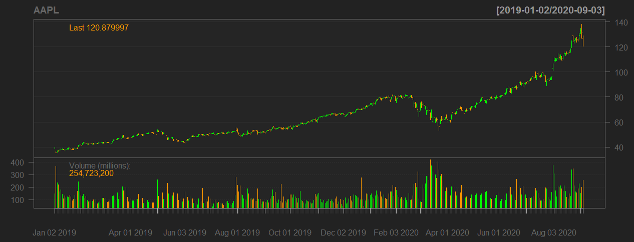
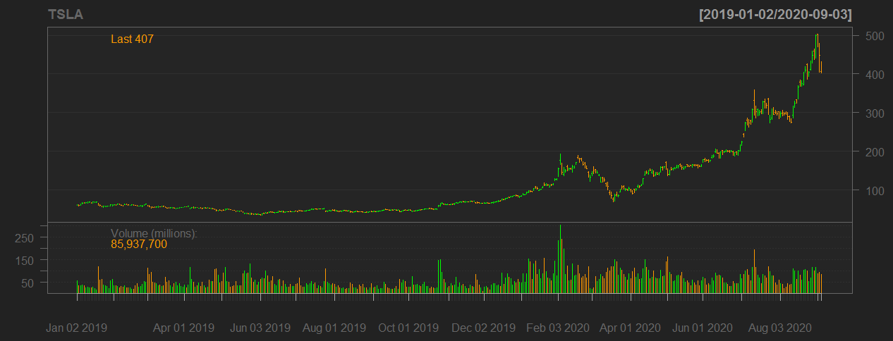
Now let’s do some visualization of our extracted data! The following code produces a financial bar chart of stock prices along with volume.

現在，讓我們對提取的數據進行一些可視化！ 以下代碼生成股票價格和數量的財務條形圖。

步驟3：創建技術指標 (Step-3: Creating Technical Indicators)

There are many technical indicators used for financial analysis but, for our analysis we are going to use six of the most famous technical indicators namely : Simple Moving Average (SMA), Parabolic Stop And Reverse (SAR), Commodity Channel Index (CCI), Rate Of Change (ROC), Stochastic Momentum Index (SMI) and finally Williams %R

有許多技術指標可用于財務分析，但在我們的分析中，我們將使用六種最著名的技術指標：簡單移動平均線(SMA)，拋物線止損和反向(SAR)，商品通道指數(CCI)，變化率(ROC)，隨機動量指數(SMI)，最后是威廉姆斯％R

Simple Moving Average (SMA) :

簡單移動平均線(SMA)：

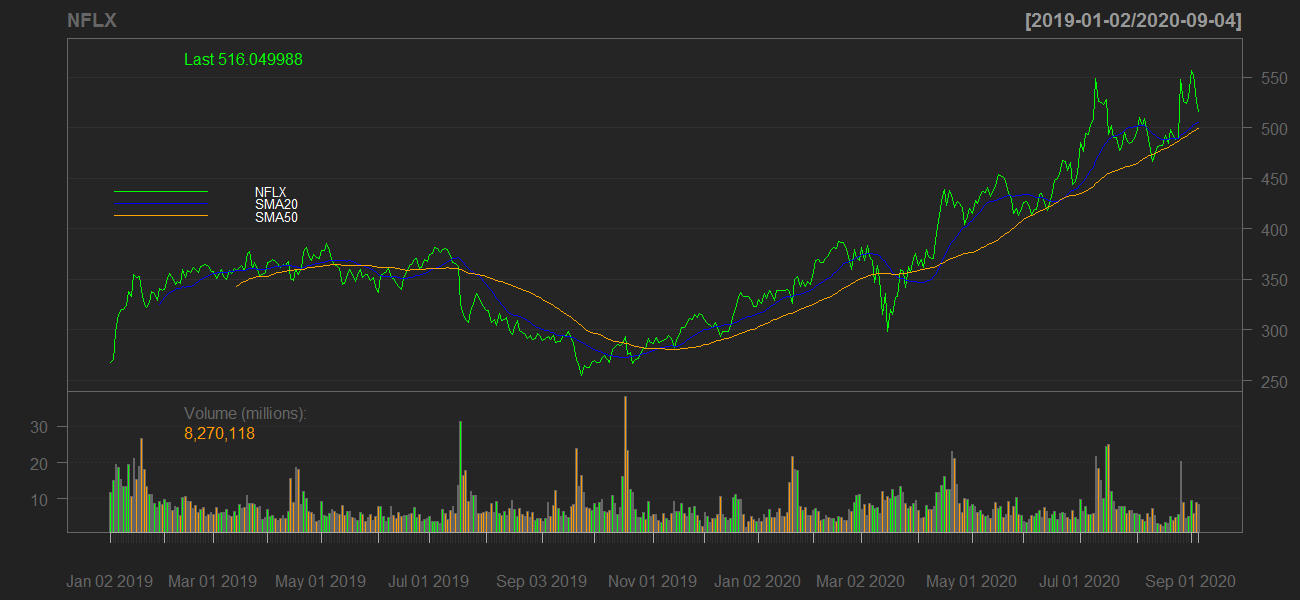
The standard interval of time we are going to use is 20 days SMA and 50 days SMA. But, there no restrictions to use any interval of time.

我們將使用的標準時間間隔是20天SMA和50天SMA。 但是，使用任何時間間隔都沒有限制。

The following code will calculate three companies’ 20 days SMA and 50 days SMA along with a plot:

以下代碼將計算三個公司的20天SMA和50天SMA以及圖表：

# 1. AAPL
sma20_aapl <- SMA(AAPL$AAPL.Close, n = 20)
sma50_aapl <- SMA(AAPL$AAPL.Close, n = 50)
lineChart(AAPL, theme = chartTheme('black'))
addSMA(n = 20, col = 'blue')
addSMA(n = 50, col = 'orange')
legend('left', col = c('green','blue','orange'),legend = c('AAPL','SMA20','SMA50'), lty = 1, bty = 'n',text.col = 'white', cex = 0.8)# 2. TSLA
sma20_tsla <- SMA(TSLA$TSLA.Close, n = 20)
sma50_tsla <- SMA(TSLA$TSLA.Close, n = 50)
lineChart(TSLA, theme = 'black')
addSMA(n = 20, col = 'blue')
addSMA(n = 50, col = 'orange')
legend('left', col = c('green','blue','orange'),legend = c('AAPL','SMA20','SMA50'), lty = 1, bty = 'n',text.col = 'white', cex = 0.8)# 3. NFLX
sma20_nflx <- SMA(NFLX$NFLX.Close, n = 20)
sma50_nflx <- SMA(NFLX$NFLX.Close, n = 50)
lineChart(NFLX, theme = 'black')
addSMA(n = 20, col = 'blue')
addSMA(n = 50, col = 'orange')
legend('left', col = c('green','blue','orange'),legend = c('AAPL','SMA20','SMA50'), lty = 1, bty = 'n',text.col = 'white', cex = 0.8)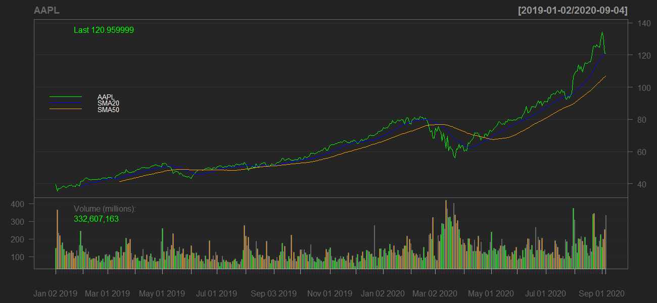

Parabolic Stop And Reverse (SAR) :

拋物線反轉(SAR)：

To calculate Parabolic SAR, we have to pass on daily High and Low prices of the companies along with a given acceleration value.

要計算拋物線比吸收率，我們必須傳遞公司的每日最高價和最低價以及給定的加速值。

The following code will calculate the companies’ Parabolic SAR along with a plot:

以下代碼將計算公司的拋物線比吸收率以及圖：

# 1. AAPL
sar_aapl <- SAR(cbind(Hi(AAPL),Lo(AAPL)), accel = c(0.02, 0.2))
barChart(AAPL, theme = 'black')
addSAR(accel = c(0.02, 0.2), col = 'lightblue')# 2. TSLA
sar_tsla <- SAR(cbind(Hi(TSLA),Lo(TSLA)), accel = c(0.02, 0.2))
barChart(TSLA, theme = 'black')
addSAR(accel = c(0.02, 0.2), col = 'lightblue')# 3. NFLX
sar_nflx <- SAR(cbind(Hi(NFLX),Lo(NFLX)), accel = c(0.02, 0.2))
barChart(NFLX, theme = 'black')
addSAR(accel = c(0.02, 0.2), col = 'lightblue')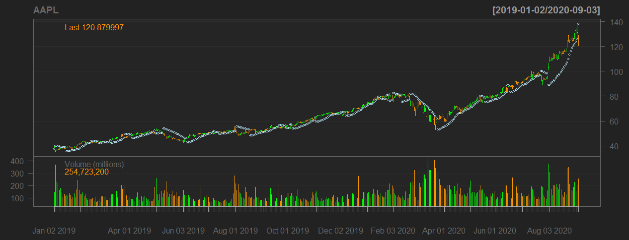

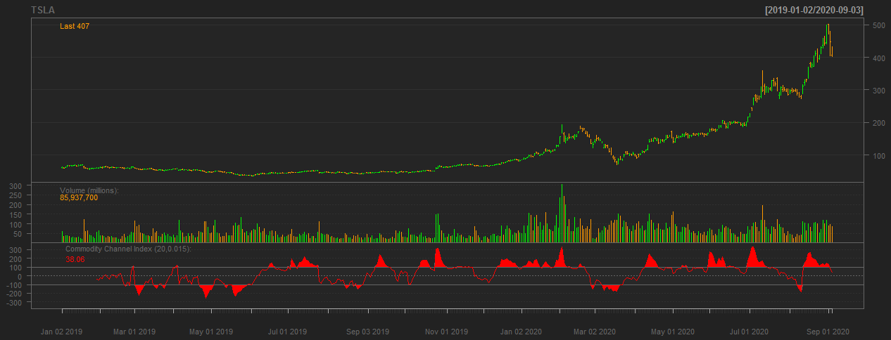
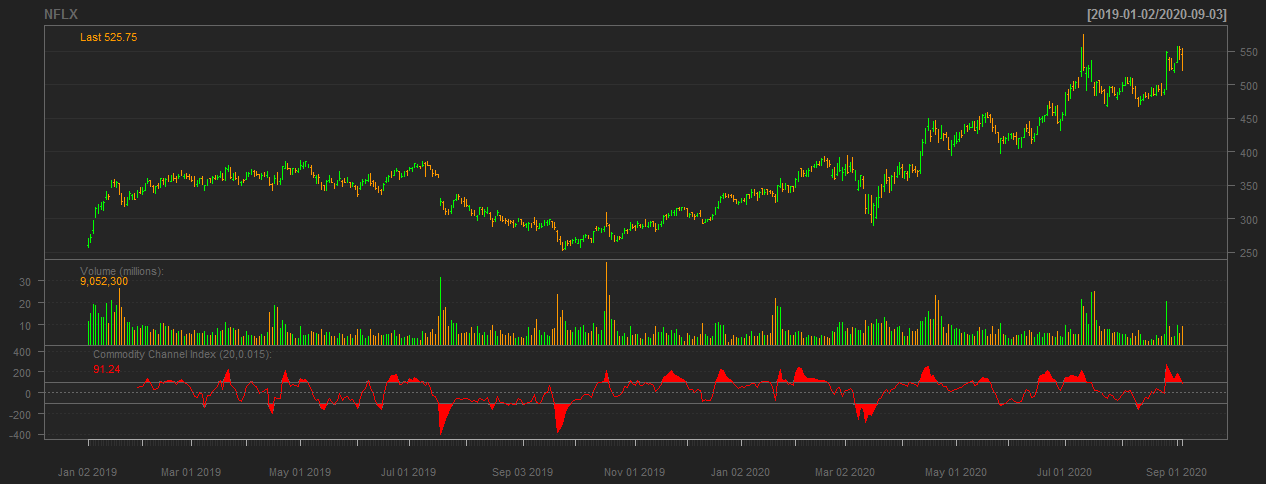
Commodity Channel Index (CCI) :

商品渠道指數(CCI)：

To calculate CCI, we have to pass on daily High, Low and Close prices of companies along with a specified time period and a constant value. In this step, we are going to take 20 days as time period and 0.015 as the constant value.

要計算CCI，我們必須傳遞公司的每日最高價，最低價和收盤價以及指定的時間段和恒定值。 在此步驟中，我們將時間段設為20天，將常數值設為0.015。

The following code will calculate the companies’ CCI along with a plot:

以下代碼將計算公司的CCI以及圖：

# 1. AAPL
cci_aapl <- CCI(HLC(AAPL), n = 20, c = 0.015)
barChart(AAPL, theme = 'black')
addCCI(n = 20, c = 0.015)# 2. TSLA
cci_tsla <- CCI(HLC(TSLA), n = 20, c = 0.015)
barChart(TSLA, theme = 'black')
addCCI(n = 20, c = 0.015)# 3. NFLX
cci_nflx <- CCI(HLC(NFLX), n = 20, c = 0.015)
barChart(NFLX, theme = 'black')
addCCI(n = 20, c = 0.015)

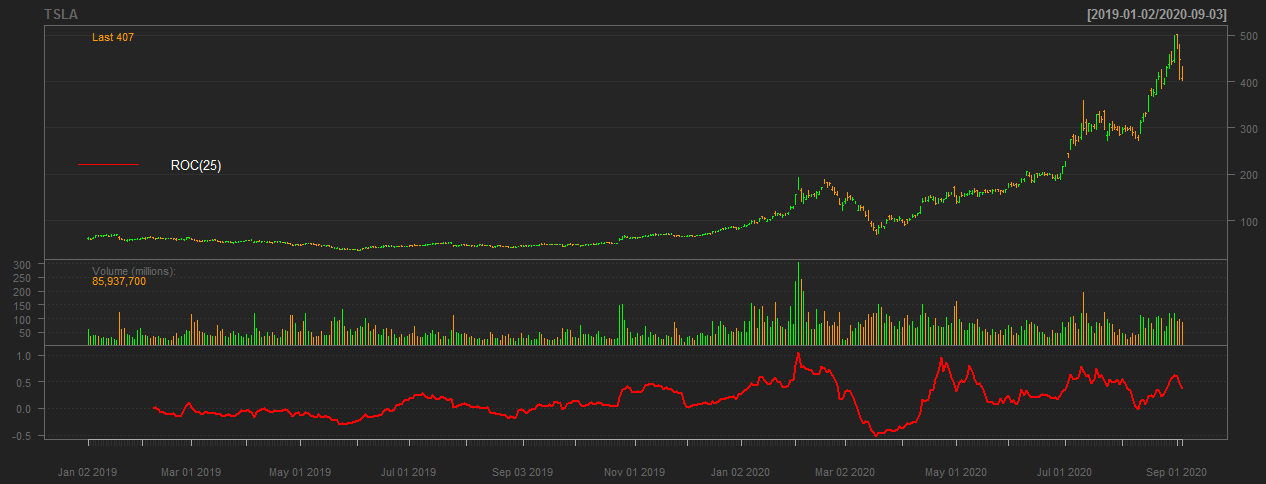
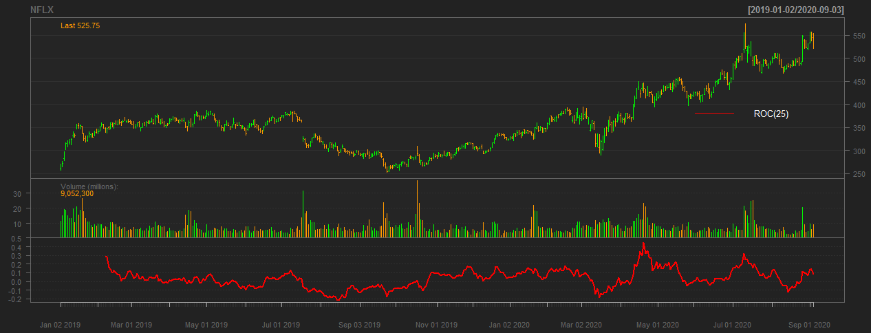
Rate Of Change (ROC)

變化率(ROC)

To calculate ROC, we have to pass on a specified interval of time and there is no restrictions in using any number of period. In this step, we are going to use 25 days as the period of time.

要計算ROC，我們必須經過指定的時間間隔，并且使用任何數量的周期都沒有限制。 在此步驟中，我們將使用25天作為時間段。

The following code will calculate the companies’ ROC along with a plot:

以下代碼將計算公司的ROC以及圖表：

# 1. AAPL
roc_aapl <- ROC(AAPL$AAPL.Close, n = 25)
barChart(AAPL, theme = 'black')
addROC(n = 25)
legend('left', col = 'red', legend = 'ROC(25)', lty = 1, bty = 'n',text.col = 'white', cex = 0.8)# 1. TSLA
roc_tsla <- ROC(TSLA$TSLA.Close, n = 25)
barChart(TSLA, theme = 'black')
addROC(n = 25)
legend('left', col = 'red', legend = 'ROC(25)', lty = 1, bty = 'n',text.col = 'white', cex = 0.8)# 1. NFLX
roc_nflx <- ROC(NFLX$NFLX.Close, n = 25)
barChart(NFLX, theme = 'black')
addROC(n = 25)
legend('right', col = 'red', legend = 'ROC(25)', lty = 1, bty = 'n',text.col = 'white', cex = 0.8)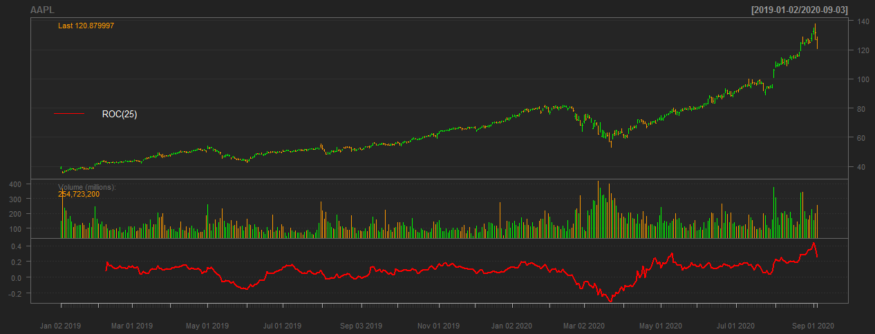

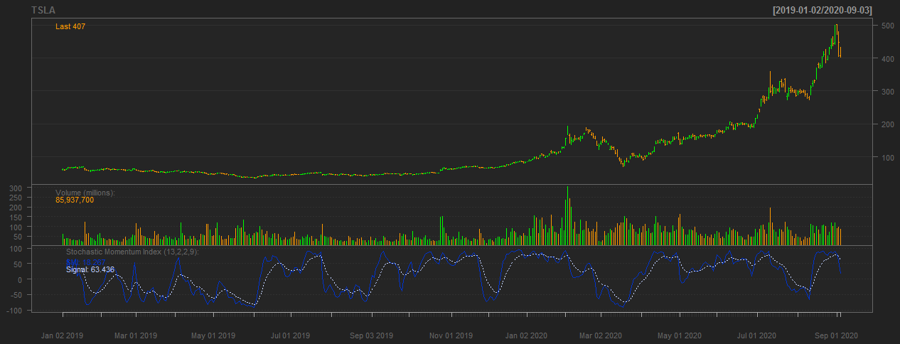
Stochastic Momentum Index (SMI) :

隨機動量指數(SMI)：

To calculate SMI, we have to pass on daily High, Low and Close prices of companies, a specified interval of time, two smoothing parameters and a signal value.

要計算SMI，我們必須傳遞公司的每日最高價，最低價和收盤價，指定的時間間隔，兩個平滑參數和一個信號值。

The following code will calculate companies’ SMI along with a plot:

以下代碼將計算公司的SMI以及圖表：

# 1. AAPL
smi_aapl <- SMI(HLC(AAPL),n = 13, nFast = 2, nSlow = 25, nSig = 9)
barChart(AAPL, theme = 'black')
addSMI(n = 13, fast = 2, slow = 2, signal = 9)# 2. TSLA
smi_tsla <- SMI(HLC(TSLA),n = 13, nFast = 2, nSlow = 25, nSig = 9)
barChart(TSLA, theme = 'black')
addSMI(n = 13, fast = 2, slow = 2, signal = 9)# 3. NFLX
smi_nflx <- SMI(HLC(NFLX),n = 13, nFast = 2, nSlow = 25, nSig = 9)
barChart(NFLX, theme = 'black')
addSMI(n = 13, fast = 2, slow = 2, signal = 9)

Williams %R

威廉姆斯％R

To calculate Williams %R, we have to pass on the daily High, Low and Close prices of companies along with a specified number of periods.

要計算Williams％R，我們必須傳遞公司的每日最高價，最低價和收盤價以及指定的期間數。

The following code will calculate the companies’ Williams %R along with a plot:

以下代碼將計算公司的Williams％R以及圖表：

# 1. AAPL
wpr_aapl <- WPR(HLC(AAPL), n = 14)
colnames(wpr_aapl) <- 'wpr'
barChart(AAPL, theme = 'black')
addWPR(n = 14)# 1. TSLA
wpr_tsla <- WPR(HLC(TSLA), n = 14)
colnames(wpr_tsla) <- 'wpr'
barChart(TSLA, theme = 'black')
addWPR(n = 14)# 1. NFLX
wpr_nflx <- WPR(HLC(NFLX), n = 14)
colnames(wpr_nflx) <- 'wpr'
barChart(NFLX, theme = 'black')
addWPR(n = 14)

步驟4：創建交易信號 (Step-4 : Creating Trading Signals)

In this step, we are going to use the previously created indicators to build ‘BUY’ or ‘SELL’ trading signals. Basically, we will pass on specific conditions and if the condition satisfies a ‘BUY’ signal our created trading signal will turn to 1 which means a buy. If the condition satisfies a ‘SELL’ signal our created trading signal will turn to -1 which means a sell. If it doesn’t satisfies any of the mentioned conditions, then it will turn to 0 which means nothing. It might sounds like a whole bunch of fuzz but, it will be clear once we dive into the coding section. After coding your trading signals, you can use the ‘which’ command in R to see how may ‘BUY’ signals and how many ‘SELL’ signals.

在這一步中，我們將使用先前創建的指標來建立“買入”或“賣出”交易信號。 基本上，我們將傳遞特定的條件，如果條件滿足“買入”信號，我們創建的交易信號將變為1，表示買入。 如果條件滿足“賣出”信號，我們創建的交易信號將變為-1，這意味著賣出。 如果不滿足上述任何條件，則它將變為0，這意味著沒有任何意義。 聽起來似乎很模糊，但是一旦我們深入到編碼部分，這一點就很清楚了。 在對交易信號進行編碼之后，您可以使用R中的“哪個”命令來查看“買入”信號的數量和“賣出”信號的數量。

Simple Moving Average

簡單移動平均線

The following code will create SMA trading signals for companies if it satisfies our given condition:

如果滿足我們的條件，以下代碼將為公司創建SMA交易信號：

# SMA # a. AAPL
# SMA 20 Crossover Signal 
sma20_aapl_ts <- Lag(ifelse(Lag(Cl(AAPL)) < Lag(sma20_aapl) & Cl(AAPL) > sma20_aapl,1,ifelse(Lag(Cl(AAPL)) > Lag(sma20_aapl) & Cl(AAPL) < sma20_aapl,-1,0)))
sma20_aapl_ts[is.na(sma20_aapl_ts)] <- 0
# SMA 50 Crossover Signal
sma50_aapl_ts <- Lag(ifelse(Lag(Cl(AAPL)) < Lag(sma50_aapl) & Cl(AAPL) > sma50_aapl,1,ifelse(Lag(Cl(AAPL)) > Lag(sma50_aapl) & Cl(AAPL) < sma50_aapl,-1,0)))
sma50_aapl_ts[is.na(sma50_aapl_ts)] <- 0
# SMA 20 and SMA 50 Crossover Signal
sma_aapl_ts <- Lag(ifelse(Lag(sma20_aapl) < Lag(sma50_aapl) & sma20_aapl > sma50_aapl,1,ifelse(Lag(sma20_aapl) > Lag(sma50_aapl) & sma20_aapl < sma50_aapl,-1,0)))
sma_aapl_ts[is.na(sma_aapl_ts)] <- 0# b. TSLA
# SMA 20 Crossover Signal 
sma20_tsla_ts <- Lag(ifelse(Lag(Cl(TSLA)) < Lag(sma20_tsla) & Cl(TSLA) > sma20_tsla,1,ifelse(Lag(Cl(TSLA)) > Lag(sma20_tsla) & Cl(TSLA) < sma20_tsla,-1,0)))
sma20_tsla_ts[is.na(sma20_tsla_ts)] <- 0
# SMA 50 Crossover Signal
sma50_tsla_ts <- Lag(ifelse(Lag(Cl(TSLA)) < Lag(sma50_tsla) & Cl(TSLA) > sma50_tsla,1,ifelse(Lag(Cl(TSLA)) > Lag(sma50_tsla) & Cl(TSLA) < sma50_tsla,-1,0)))
sma50_tsla_ts[is.na(sma50_tsla_ts)] <- 0
# SMA 20 and SMA 50 Crossover Signal
sma_tsla_ts <- Lag(ifelse(Lag(sma20_tsla) < Lag(sma50_tsla) & sma20_tsla > sma50_tsla,1,ifelse(Lag(sma20_tsla) > Lag(sma50_tsla) & sma20_tsla < sma50_tsla,-1,0)))
sma_tsla_ts[is.na(sma_tsla_ts)] <- 0# c. NFLX
# SMA 20 Crossover Signal 
sma20_nflx_ts <- Lag(ifelse(Lag(Cl(NFLX)) < Lag(sma20_nflx) & Cl(NFLX) > sma20_nflx,1,ifelse(Lag(Cl(NFLX)) > Lag(sma20_nflx) & Cl(NFLX) < sma20_nflx,-1,0)))
sma20_nflx_ts[is.na(sma20_nflx_ts)] <- 0
# SMA 50 Crossover Signal
sma50_nflx_ts <- Lag(ifelse(Lag(Cl(NFLX)) < Lag(sma50_nflx) & Cl(NFLX) > sma50_nflx,1,ifelse(Lag(Cl(NFLX)) > Lag(sma50_nflx) & Cl(NFLX) < sma50_nflx,-1,0)))
sma50_nflx_ts[is.na(sma50_nflx_ts)] <- 0
# SMA 20 and SMA 50 Crossover Signal
sma_nflx_ts <- Lag(ifelse(Lag(sma20_nflx) < Lag(sma50_nflx) & sma20_nflx > sma50_nflx,1,ifelse(Lag(sma20_nflx) > Lag(sma50_nflx) & sma20_nflx < sma50_nflx,-1,0)))
sma_nflx_ts[is.na(sma_nflx_ts)] <- 0

Parabolic Stop and Reverse (SAR)

拋物線停止和反向(SAR)

The following code will create Parabolic SAR trading signal for companies if it satisfies our conditions:

如果滿足我們的條件，以下代碼將為公司創建拋物線SAR交易信號：

# Parabolic Stop And Reverse (SAR) # a. AAPL
sar_aapl_ts <- Lag(ifelse(Lag(Cl(AAPL)) < Lag(sar_aapl) & Cl(AAPL) > sar_aapl,1,ifelse(Lag(Cl(AAPL)) > Lag(sar_aapl) & Cl(AAPL) < sar_aapl,-1,0)))
sar_aapl_ts[is.na(sar_aapl_ts)] <- 0# b. TSLA
sar_tsla_ts <- Lag(ifelse(Lag(Cl(TSLA)) < Lag(sar_tsla) & Cl(TSLA) > sar_tsla,1,ifelse(Lag(Cl(TSLA)) > Lag(sar_tsla) & Cl(TSLA) < sar_tsla,-1,0)))
sar_tsla_ts[is.na(sar_tsla_ts)] <- 0# c. NFLX
sar_nflx_ts <- Lag(ifelse(Lag(Cl(NFLX)) < Lag(sar_nflx) & Cl(NFLX) > sar_nflx,1,ifelse(Lag(Cl(NFLX)) > Lag(sar_nflx) & Cl(NFLX) < sar_nflx,-1,0)))
sar_nflx_ts[is.na(sar_nflx_ts)] <- 0

Commodity Channel Index (CCI)

商品渠道指數(CCI)

The following code will create CCI trading signals for companies if it satisfies our conditions:

如果滿足我們的條件，以下代碼將為公司創建CCI交易信號：

# Commodity Channel Index  (CCI)# a. AAPL
cci_aapl_ts <- Lag(ifelse(Lag(cci_aapl) < (-100) & cci_aapl > (-100),1,ifelse(Lag(cci_aapl) < (100) & cci_aapl > (100),-1,0)))
cci_aapl_ts[is.na(cci_aapl_ts)] <- 0# b. TSLA
cci_tsla_ts <- Lag(ifelse(Lag(cci_tsla) < (-100) & cci_tsla > (-100),1,ifelse(Lag(cci_tsla) < (100) & cci_tsla > (100),-1,0)))
cci_tsla_ts[is.na(cci_tsla_ts)] <- 0# c. NFLX
cci_nflx_ts <- Lag(ifelse(Lag(cci_nflx) < (-100) & cci_nflx > (-100),1,ifelse(Lag(cci_nflx) < (100) & cci_nflx > (100),-1,0)))
cci_nflx_ts[is.na(cci_nflx_ts)] <- 0

Rate of Change (ROC)

變化率(ROC)

The following code will create Rate Of Change (ROC) trading signals for companies if it satisfies our conditions:

如果滿足我們的條件，以下代碼將為公司創建更改率(ROC)交易信號：

# Rate of Change (ROC)# a. AAPL
roc_aapl_ts <- Lag(ifelse(Lag(roc_aapl) < (-0.05) & roc_aapl > (-0.05),1,ifelse(Lag(roc_aapl) < (0.05) & roc_aapl > (0.05),-1,0)))
roc_aapl_ts[is.na(roc_aapl_ts)] <- 0# b. TSLA
roc_tsla_ts <- Lag(ifelse(Lag(roc_tsla) < (-0.05) & roc_tsla > (-0.05),1,ifelse(Lag(roc_tsla) < (0.05) & roc_tsla > (0.05),-1,0)))
roc_tsla_ts[is.na(roc_tsla_ts)] <- 0# c. NFLX
roc_nflx_ts <- Lag(ifelse(Lag(roc_nflx) < (-0.05) & roc_nflx > (-0.05),1,ifelse(Lag(roc_nflx) < (0.05) & roc_nflx > (0.05),-1,0)))
roc_nflx_ts[is.na(roc_nflx_ts)] <- 0

Stochastic Momentum Index (SMI)

隨機動量指數(SMI)

The following code will create Stochastic Momentum Index (SMI) trading signals for companies if it satisfies our conditions:

如果滿足我們的條件，以下代碼將為公司創建隨機動量指數(SMI)交易信號：

# Stochastic Momentum Index (SMI)# a. AAPL
smi_aapl_ts <- Lag(ifelse(Lag(smi_aapl[,1]) < Lag(smi_aapl[,2]) & smi_aapl[,1] > smi_aapl[,2],1, ifelse(Lag(smi_aapl[,1]) > Lag(smi_aapl[,2]) & smi_aapl[,1] < smi_aapl[,2],-1,0)))
smi_aapl_ts[is.na(smi_aapl_ts)] <- 0# b. TSLA
smi_tsla_ts <- Lag(ifelse(Lag(smi_tsla[,1]) < Lag(smi_tsla[,2]) & smi_tsla[,1] > smi_tsla[,2],1, ifelse(Lag(smi_tsla[,1]) > Lag(smi_tsla[,2]) & smi_tsla[,1] < smi_tsla[,2],-1,0)))
smi_tsla_ts[is.na(smi_tsla_ts)] <- 0# a. NFLX
smi_nflx_ts <- Lag(ifelse(Lag(smi_nflx[,1]) < Lag(smi_nflx[,2]) & smi_nflx[,1] > smi_nflx[,2],1, ifelse(Lag(smi_nflx[,1]) > Lag(smi_nflx[,2]) & smi_nflx[,1] < smi_nflx[,2],-1,0)))
smi_nflx_ts[is.na(smi_nflx_ts)] <- 0

Williams %R

威廉姆斯％R

The following code will create Williams %R trading signals for companies if it satisfies our conditions:

如果滿足我們的條件，以下代碼將為公司創建Williams％R交易信號：

# Williams %R# a. AAPL
wpr_aapl_ts <- Lag(ifelse(Lag(wpr_aapl) > 0.8 & wpr_aapl < 0.8,1,ifelse(Lag(wpr_aapl) > 0.2 & wpr_aapl < 0.2,-1,0)))
wpr_aapl_ts[is.na(wpr_aapl_ts)] <- 0# b. TSLA
wpr_tsla_ts <- Lag(ifelse(Lag(wpr_tsla) > 0.8 & wpr_tsla < 0.8,1,ifelse(Lag(wpr_tsla) > 0.2 & wpr_tsla < 0.2,-1,0)))
wpr_tsla_ts[is.na(wpr_tsla_ts)] <- 0# c. NFLX
wpr_nflx_ts <- Lag(ifelse(Lag(wpr_nflx) > 0.8 & wpr_nflx < 0.8,1,ifelse(Lag(wpr_nflx) > 0.2 & wpr_nflx < 0.2,-1,0)))
wpr_nflx_ts[is.na(wpr_nflx_ts)] <- 0

步驟5：制定交易策略 (Step-5 : Creating Trading Strategies)

This is the most interesting step in our process as we are going to create Trading Strategies using our previously created Trading Signals. In our previous step, we created signals whether to buy or sell and in this step we are going to create conditions to check our holding position in that stock (i.e., whether we hold, bought or sold the stock). The trading strategy we are about to code will return 1 if we hold the stock or returns 0 if we don’t own the stock.

這是我們流程中最有趣的步驟，因為我們將使用先前創建的交易信號來創建交易策略。 在上一步中，我們創建了買入或賣出信號，在這一步中，我們將創建條件來檢查我們在該股票中的持倉狀況(即我們是否持有，買入或賣出該股票)。 如果我們持有股票，我們將要編碼的交易策略將返回1；如果我們不擁有股票，則將返回0。

Simple Moving Average

簡單移動平均線

The following code will create a SMA trading strategy if satisfies our given conditions:

如果滿足我們的條件，以下代碼將創建SMA交易策略：

# SMA 20 and SMA 50 Crossover Strategy# a. AAPLsma_aapl_strat <- ifelse(sma_aapl_ts > 1,0,1)
for (i in 1 : length(Cl(AAPL))) {sma_aapl_strat[i] <- ifelse(sma_aapl_ts[i] == 1,1,ifelse(sma_aapl_ts[i] == -1,0,sma_aapl_strat[i-1]))
}
sma_aapl_strat[is.na(sma_aapl_strat)] <- 1
sma_aapl_stratcomp <- cbind(sma20_aapl, sma50_aapl, sma_aapl_ts, sma_aapl_strat)
colnames(sma_aapl_stratcomp) <- c('SMA(20)','SMA(50)','SMA SIGNAL','SMA POSITION')# b. TSLA
sma_tsla_strat <- ifelse(sma_tsla_ts > 1,0,1)
for (i in 1 : length(Cl(TSLA))) {sma_tsla_strat[i] <- ifelse(sma_tsla_ts[i] == 1,1,ifelse(sma_tsla_ts[i] == -1,0,sma_tsla_strat[i-1]))
}
sma_tsla_strat[is.na(sma_tsla_strat)] <- 1
sma_tsla_stratcomp <- cbind(sma20_tsla, sma50_tsla, sma_tsla_ts, sma_tsla_strat)
colnames(sma_tsla_stratcomp) <- c('SMA(20)','SMA(50)','SMA SIGNAL','SMA POSITION')# c. NFLX
sma_nflx_strat <- ifelse(sma_nflx_ts > 1,0,1)
for (i in 1 : length(Cl(NFLX))) {sma_nflx_strat[i] <- ifelse(sma_nflx_ts[i] == 1,1,ifelse(sma_nflx_ts[i] == 'SEL',0,sma_nflx_strat[i-1]))
}
sma_nflx_strat[is.na(sma_nflx_strat)] <- 1
sma_nflx_stratcomp <- cbind(sma20_nflx, sma50_nflx, sma_nflx_ts, sma_nflx_strat)
colnames(sma_nflx_stratcomp) <- c('SMA(20)','SMA(50)','SMA SIGNAL','SMA POSITION')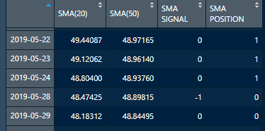

This is an example table of our created SMA Apple trading strategy. In this table we can observe that, on 2019–05–24 SMA 20 went below SMA 50 so our created signal returns -1 (‘SELL’) the next day also our position changes to 0 which means we don’t hold the stock. From this, we can say that our created strategy works as we expected. Now, let’s proceed to the remaining Trading Strategies.

這是我們創建的SMA Apple交易策略的示例表。 在此表中，我們可以觀察到，在2019–05–24 SMA 20低于SMA 50，因此我們創建的信號在第二天返回-1(“賣出”)，我們的頭寸也變為0，這意味著我們不持有股票。 由此，我們可以說我們創建的策略可以按預期工作。 現在，讓我們繼續其余的交易策略。

Parabolic Stop And Reverse (SAR)

拋物線停止和反轉(SAR)

The following code will create a Parabolic SAR trading strategy if satisfies our given conditions:

如果滿足我們的條件，以下代碼將創建拋物線形SAR交易策略：

# Parabolic SAR Strategy # a. AAPL
sar_aapl_strat <- ifelse(sar_aapl_ts > 1,0,1)
for (i in 1 : length(Cl(AAPL))) {sar_aapl_strat[i] <- ifelse(sar_aapl_ts[i] == 1,1,ifelse(sar_aapl_ts[i] == -1,0,sar_aapl_strat[i-1]))
}
sar_aapl_strat[is.na(sar_aapl_strat)] <- 1
sar_aapl_stratcomp <- cbind(Cl(AAPL), sar_aapl, sar_aapl_ts, sar_aapl_strat)
colnames(sar_aapl_stratcomp) <- c('Close','SAR','SAR SIGNAL','SAR POSITION')# b. TSLA
sar_tsla_strat <- ifelse(sar_tsla_ts > 1,0,1)
for (i in 1 : length(Cl(TSLA))) {sar_tsla_strat[i] <- ifelse(sar_tsla_ts[i] == 1,1,ifelse(sar_tsla_ts[i] == -1,0,sar_tsla_strat[i-1]))
}
sar_tsla_strat[is.na(sar_tsla_strat)] <- 1
sar_tsla_stratcomp <- cbind(Cl(TSLA), sar_tsla, sar_tsla_ts, sar_tsla_strat)
colnames(sar_tsla_stratcomp) <- c('Close','SAR','SAR SIGNAL','SAR POSITION')# c. NFLX
sar_nflx_strat <- ifelse(sar_nflx_ts > 1,0,1)
for (i in 1 : length(Cl(NFLX))) {sar_nflx_strat[i] <- ifelse(sar_nflx_ts[i] == 1,1,ifelse(sar_nflx_ts[i] == -1,0,sar_nflx_strat[i-1]))
}
sar_nflx_strat[is.na(sar_nflx_strat)] <- 1
sar_nflx_stratcomp <- cbind(Cl(NFLX), sar_nflx, sar_nflx_ts, sar_nflx_strat)
colnames(sar_nflx_stratcomp) <- c('Close','SAR','SAR SIGNAL','SAR POSITION')

Commodity Channel Index (CCI) :

商品渠道指數(CCI)：

The following code will create a CCI trading strategy if satisfies our given conditions:

如果滿足我們的條件，以下代碼將創建CCI交易策略：

# CCI# a. AAPL
cci_aapl_strat <- ifelse(cci_aapl_ts > 1,0,1)
for (i in 1 : length(Cl(AAPL))) {cci_aapl_strat[i] <- ifelse(cci_aapl_ts[i] == 1,1,ifelse(cci_aapl_ts[i] == -1,0,cci_aapl_strat[i-1]))
}
cci_aapl_strat[is.na(cci_aapl_strat)] <- 1
cci_aapl_stratcomp <- cbind(cci_aapl, cci_aapl_ts, cci_aapl_strat)
colnames(cci_aapl_stratcomp) <- c('CCI','CCI SIGNAL','CCI POSITION')# b. TSLA
cci_tsla_strat <- ifelse(cci_tsla_ts > 1,0,1)
for (i in 1 : length(Cl(TSLA))) {cci_tsla_strat[i] <- ifelse(cci_tsla_ts[i] == 1,1,ifelse(cci_tsla_ts[i] == -1,0,cci_tsla_strat[i-1]))
}
cci_tsla_strat[is.na(cci_tsla_strat)] <- 1
cci_tsla_stratcomp <- cbind(cci_tsla, cci_tsla_ts, cci_tsla_strat)
colnames(cci_tsla_stratcomp) <- c('CCI','CCI SIGNAL','CCI POSITION')# c. NFLX
cci_nflx_strat <- ifelse(cci_nflx_ts > 1,0,1)
for (i in 1 : length(Cl(NFLX))) {cci_nflx_strat[i] <- ifelse(cci_nflx_ts[i] == 1,1,ifelse(cci_nflx_ts[i] == -1,0,cci_nflx_strat[i-1]))
}
cci_nflx_strat[is.na(cci_nflx_strat)] <- 1
cci_nflx_stratcomp <- cbind(cci_nflx, cci_nflx_ts, cci_nflx_strat)
colnames(cci_nflx_stratcomp) <- c('CCI','CCI SIGNAL','CCI POSITION')

Rate Of Change (ROC)

變化率(ROC)

The following code will create a Rate Of Change (ROC) trading strategy if satisfies our given conditions:

如果滿足我們的給定條件，以下代碼將創建一個變化率(ROC)交易策略：

# ROC# a. AAPL
roc_aapl_strat <- ifelse(roc_aapl_ts > 1,0,1)
for (i in 1 : length(Cl(AAPL))) {roc_aapl_strat[i] <- ifelse(roc_aapl_ts[i] == 1,1,ifelse(roc_aapl_ts[i] == -1,0,roc_aapl_strat[i-1]))
}
roc_aapl_strat[is.na(roc_aapl_strat)] <- 1
roc_aapl_stratcomp <- cbind(roc_aapl, roc_aapl_ts, roc_aapl_strat)
colnames(roc_aapl_stratcomp) <- c('ROC(25)','ROC SIGNAL','ROC POSITION')# b. TSLA
roc_tsla_strat <- ifelse(roc_tsla_ts > 1,0,1)
for (i in 1 : length(Cl(TSLA))) {roc_tsla_strat[i] <- ifelse(roc_tsla_ts[i] == 1,1,ifelse(roc_tsla_ts[i] == -1,0,roc_tsla_strat[i-1]))
}
roc_tsla_strat[is.na(roc_tsla_strat)] <- 1
roc_tsla_stratcomp <- cbind(roc_tsla, roc_tsla_ts, roc_tsla_strat)
colnames(roc_tsla_stratcomp) <- c('ROC(25)','ROC SIGNAL','ROC POSITION')# c. NFLX
roc_nflx_strat <- ifelse(roc_nflx_ts > 1,0,1)
for (i in 1 : length(Cl(NFLX))) {roc_nflx_strat[i] <- ifelse(roc_nflx_ts[i] == 1,1,ifelse(roc_nflx_ts[i] == -1,0,roc_nflx_strat[i-1]))
}
roc_nflx_strat[is.na(roc_nflx_strat)] <- 1
roc_nflx_stratcomp <- cbind(roc_nflx, roc_nflx_ts, roc_nflx_strat)
colnames(roc_nflx_stratcomp) <- c('ROC(25)','ROC SIGNAL','ROC POSITION')

Stochastic Momentum Index (SMI)

隨機動量指數(SMI)

The following code will create a SMI trading strategy if it satisfies our given conditions:

如果滿足我們的條件，以下代碼將創建一個SMI交易策略：

# SMI# a. AAPL
smi_aapl_strat <- ifelse(smi_aapl_ts > 1,0,1)
for (i in 1 : length(Cl(AAPL))) {smi_aapl_strat[i] <- ifelse(smi_aapl_ts[i] == 1,1,ifelse(smi_aapl_ts[i] == -1,0,smi_aapl_strat[i-1]))
}
smi_aapl_strat[is.na(smi_aapl_strat)] <- 1
smi_aapl_stratcomp <- cbind(smi_aapl[,1],smi_aapl[,2],smi_aapl_ts,smi_aapl_strat)
colnames(smi_aapl_stratcomp) <- c('SMI','SMI(S)','SMI SIGNAL','SMI POSITION')# b. TSLA
smi_tsla_strat <- ifelse(smi_tsla_ts > 1,0,1)
for (i in 1 : length(Cl(TSLA))) {smi_tsla_strat[i] <- ifelse(smi_tsla_ts[i] == 1,1,ifelse(smi_tsla_ts[i] == -1,0,smi_tsla_strat[i-1]))
}
smi_tsla_strat[is.na(smi_tsla_strat)] <- 1
smi_tsla_stratcomp <- cbind(smi_tsla[,1],smi_tsla[,2],smi_tsla_ts,smi_tsla_strat)
colnames(smi_tsla_stratcomp) <- c('SMI','SMI(S)','SMI SIGNAL','SMI POSITION')# c. NFLX
smi_nflx_strat <- ifelse(smi_nflx_ts > 1,0,1)
for (i in 1 : length(Cl(NFLX))) {smi_nflx_strat[i] <- ifelse(smi_nflx_ts[i] == 1,1,ifelse(smi_nflx_ts[i] == -1,0,smi_nflx_strat[i-1]))
}
smi_nflx_strat[is.na(smi_nflx_strat)] <- 1
smi_nflx_stratcomp <- cbind(smi_nflx[,1],smi_nflx[,2],smi_nflx_ts,smi_nflx_strat)
colnames(smi_nflx_stratcomp) <- c('SMI','SMI(S)','SMI SIGNAL','SMI POSITION')

Williams %R

威廉姆斯％R

The following code will create a Williams %R trading strategy if it satisfies our given conditions:

如果滿足我們給定的條件，以下代碼將創建Williams％R交易策略：

# WPR# a. AAPL
wpr_aapl_strat <- ifelse(wpr_aapl_ts > 1,0,1)
for (i in 1 : length(Cl(AAPL))) {wpr_aapl_strat[i] <- ifelse(wpr_aapl_ts[i] == 1,1,ifelse(wpr_aapl_ts[i] == -1,0,wpr_aapl_strat[i-1]))
}
wpr_aapl_strat[is.na(wpr_aapl_strat)] <- 1
wpr_aapl_stratcomp <- cbind(wpr_aapl, wpr_aapl_ts, wpr_aapl_strat)
colnames(wpr_aapl_stratcomp) <- c('WPR(14)','WPR SIGNAL','WPR POSITION')# b. TSLA
wpr_tsla_strat <- ifelse(wpr_tsla_ts > 1,0,1)
for (i in 1 : length(Cl(TSLA))) {wpr_tsla_strat[i] <- ifelse(wpr_tsla_ts[i] == 1,1,ifelse(wpr_tsla_ts[i] == -1,0,wpr_tsla_strat[i-1]))
}
wpr_tsla_strat[is.na(wpr_tsla_strat)] <- 1
wpr_tsla_stratcomp <- cbind(wpr_tsla, wpr_tsla_ts, wpr_tsla_strat)
colnames(wpr_tsla_stratcomp) <- c('WPR(14)','WPR SIGNAL','WPR POSITION')# c. NFLX
wpr_nflx_strat <- ifelse(wpr_nflx_ts > 1,0,1)
for (i in 1 : length(Cl(NFLX))) {wpr_nflx_strat[i] <- ifelse(wpr_nflx_ts[i] == 1,1,ifelse(wpr_nflx_ts[i] == -1,0,wpr_nflx_strat[i-1]))
}
wpr_nflx_strat[is.na(wpr_nflx_strat)] <- 1
wpr_nflx_stratcomp <- cbind(wpr_nflx, wpr_nflx_ts, wpr_nflx_strat)
colnames(wpr_nflx_stratcomp) <- c('WPR(14)','WPR SIGNAL','WPR POSITION')

步驟6：回測和比較結果 (Step-6 : Backtesting and Comparing the Results)

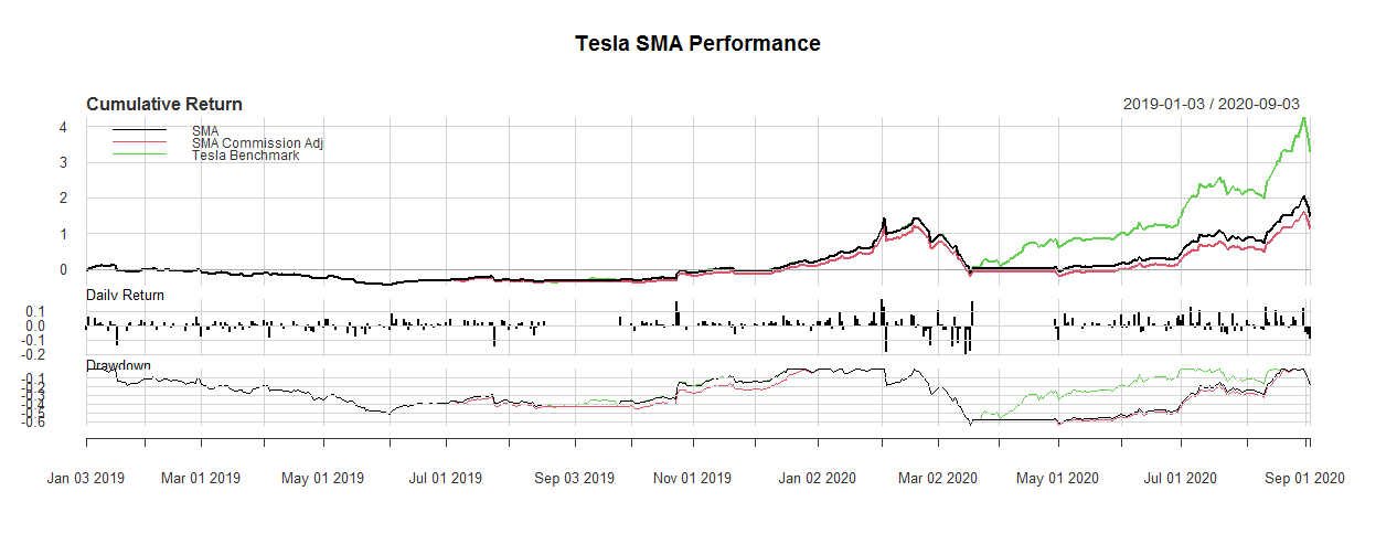
In this step we are going to conduct backtests on our created trading strategies vs our created trading strategies commission adjusted (0.5%) vs the companies’ benchmark returns. Before conducting our backtests, we have calculate our daily benchmark returns i.e., daily returns of Apple, Tesla and Netflix. Let’s do it!

在 此步驟中，我們將對我們創建的交易策略與調整后的交易策略傭金(0.5％)與公司的基準收益進行回測。 在進行回測之前，我們已經計算了每日基準回報，即Apple，Tesla和Netflix的每日回報。 我們開始做吧！

# Calculating Returns & setting Benchmark for companiesret_aapl <- diff(log(Cl(AAPL)))
ret_tsla <- diff(log(Cl(TSLA)))
ret_nflx <- diff(log(Cl(NFLX)))benchmark_aapl <- ret_aapl
benchmark_tsla <- ret_tsla
benchmark_nflx <- ret_nflx

Now, we are set to conduct our backtests.

現在，我們準備進行回測。

Simple Moving Average (SMA)

簡單移動平均線(SMA)

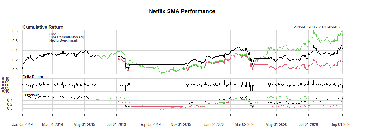
The following code will first calculate SMA strategy daily returns, commission adjusted SMA daily returns and finally runs the backtest (Comparison chart and an Annualized returns table) :

以下代碼將首先計算SMA策略的每日收益，傭金調整后的SMA日收益，最后運行回溯測試(比較圖和年化收益表)：

# SMA # 1. AAPL
sma_aapl_ret <- ret_aapl*sma_aapl_strat
sma_aapl_ret_commission_adj <- ifelse((sma_aapl_ts == 1|sma_aapl_ts == -1) & sma_aapl_strat != Lag(sma_aapl_ts), (ret_aapl-0.05)*sma_aapl_strat, ret_aapl*sma_aapl_strat)
sma_aapl_comp <- cbind(sma_aapl_ret, sma_aapl_ret_commission_adj, benchmark_aapl)
colnames(sma_aapl_comp) <- c('SMA','SMA Commission Adj','Apple Benchmark')
charts.PerformanceSummary(sma_aapl_comp, main = 'Apple SMA Performance')
sma_aapl_comp_table <- table.AnnualizedReturns(sma_aapl_comp)# 2. TSLA
sma_tsla_ret <- ret_tsla*sma_tsla_strat
sma_tsla_ret_commission_adj <- ifelse((sma_tsla_ts == 1|sma_tsla_ts == -1) & sma_tsla_strat != Lag(sma_tsla_ts), (ret_tsla-0.05)*sma_tsla_strat, ret_tsla*sma_tsla_strat)
sma_tsla_comp <- cbind(sma_tsla_ret, sma_tsla_ret_commission_adj, benchmark_tsla)
colnames(sma_tsla_comp) <- c('SMA','SMA Commission Adj','Tesla Benchmark')
charts.PerformanceSummary(sma_tsla_comp, main = 'Tesla SMA Performance')
sma_tsla_comp_table <- table.AnnualizedReturns(sma_tsla_comp)# 3. NFLX
sma_nflx_ret <- ret_nflx*sma_nflx_strat
sma_nflx_ret_commission_adj <- ifelse((sma_nflx_ts == 1|sma_nflx_ts == -1) & sma_nflx_strat != Lag(sma_nflx_ts), (ret_nflx-0.05)*sma_nflx_strat, ret_nflx*sma_nflx_strat)
sma_nflx_comp <- cbind(sma_nflx_ret, sma_nflx_ret_commission_adj, benchmark_nflx)
colnames(sma_nflx_comp) <- c('SMA','SMA Commission Adj','Netflix Benchmark')
charts.PerformanceSummary(sma_nflx_comp, main = 'Netflix SMA Performance')
sma_nflx_comp_table <- table.AnnualizedReturns(sma_nflx_comp)

Parabolic SAR

拋物線SAR

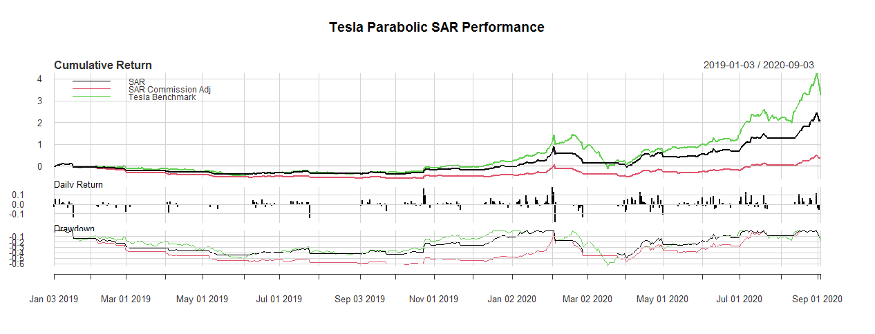
The following code will first calculate Parabolic SAR strategy daily returns, commission adjusted Parabolic SAR daily returns and finally runs the backtest (Comparison chart and an Annualized returns table) :

以下代碼將首先計算拋物線SAR策略的每日收益，傭金調整后的拋物線SAR每日收益，最后運行回測(比較圖和年度收益表)：

# Parabolic SAR # 1. AAPL
sar_aapl_ret <- ret_aapl*sar_aapl_strat
sar_aapl_ret_commission_adj <- ifelse((sar_aapl_ts == 1|sar_aapl_ts == -1) & sar_aapl_strat != Lag(sar_aapl_ts), (ret_aapl-0.05)*sar_aapl_strat, ret_aapl*sar_aapl_strat)
sar_aapl_comp <- cbind(sar_aapl_ret, sar_aapl_ret_commission_adj, benchmark_aapl)
colnames(sar_aapl_comp) <- c('SAR','SAR Commission Adj','Apple Benchmark')
charts.PerformanceSummary(sar_aapl_comp, main = 'Apple Parabolic SAR Performance')
sar_aapl_comp_table <- table.AnnualizedReturns(sar_aapl_comp)# 2. TSLA
sar_tsla_ret <- ret_tsla*sar_tsla_strat
sar_tsla_ret_commission_adj <- ifelse((sar_tsla_ts == 1|sar_tsla_ts == -1) & sar_tsla_strat != Lag(sar_tsla_ts), (ret_tsla-0.05)*sar_tsla_strat, ret_tsla*sar_tsla_strat)
sar_tsla_comp <- cbind(sar_tsla_ret, sar_tsla_ret_commission_adj, benchmark_tsla)
colnames(sar_tsla_comp) <- c('SAR','SAR Commission Adj','Tesla Benchmark')
charts.PerformanceSummary(sar_tsla_comp, main = 'Tesla Parabolic SAR Performance')
sar_tsla_comp_table <- table.AnnualizedReturns(sar_tsla_comp)# 3. NFLX
sar_nflx_ret <- ret_nflx*sar_nflx_strat
sar_nflx_ret_commission_adj <- ifelse((sar_nflx_ts == 1|sar_nflx_ts == -1) & sar_nflx_strat != Lag(sar_nflx_ts), (ret_nflx-0.05)*sar_nflx_strat, ret_nflx*sar_nflx_strat)
sar_nflx_comp <- cbind(sar_nflx_ret, sar_nflx_ret_commission_adj, benchmark_nflx)
colnames(sar_nflx_comp) <- c('SAR','SAR Commission Adj','Netflix Benchmark')
charts.PerformanceSummary(sar_nflx_comp, main = 'Netflix Parabolic SAR Performance')
sar_nflx_comp_table <- table.AnnualizedReturns(sar_nflx_comp)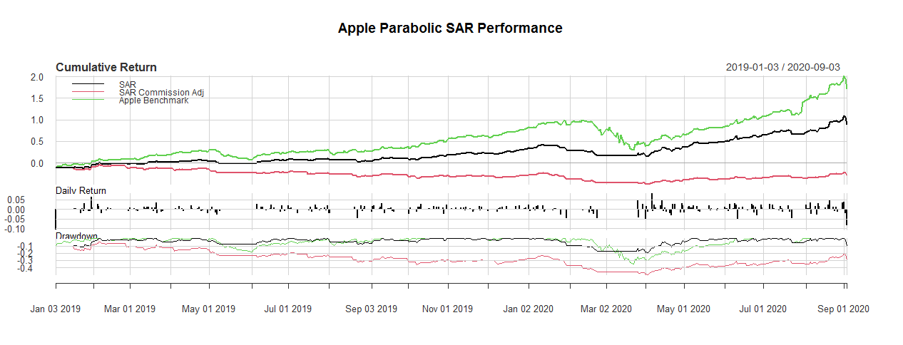

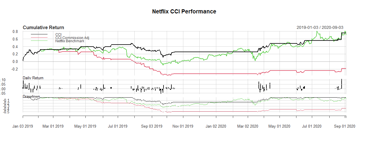
Commodity Channel Index (CCI)

商品渠道指數(CCI)

The following code will first calculate CCI strategy daily returns, commission adjusted CCI daily returns and finally runs the backtest (Comparison chart and an Annualized returns table) :

以下代碼將首先計算CCI戰略每日收益，傭金調整后的CCI日收益，最后運行回溯測試(比較圖和年化收益表)：

# CCI  # 1. AAPL
cci_aapl_ret <- ret_aapl*cci_aapl_strat
cci_aapl_ret_commission_adj <- ifelse((cci_aapl_ts == 1|cci_aapl_ts == -1) & cci_aapl_strat != Lag(cci_aapl_ts), (ret_aapl-0.05)*cci_aapl_strat, ret_aapl*cci_aapl_strat)
cci_aapl_comp <- cbind(cci_aapl_ret, cci_aapl_ret_commission_adj, benchmark_aapl)
colnames(cci_aapl_comp) <- c('CCI','CCI Commission Adj','Apple Benchmark')
charts.PerformanceSummary(cci_aapl_comp, main = 'Apple CCI Performance')
cci_aapl_comp_table <- table.AnnualizedReturns(cci_aapl_comp)# 2. TSLA
cci_tsla_ret <- ret_tsla*cci_tsla_strat
cci_tsla_ret_commission_adj <- ifelse((cci_tsla_ts == 1|cci_tsla_ts == -1) & cci_tsla_strat != Lag(cci_tsla_ts), (ret_tsla-0.05)*cci_tsla_strat, ret_tsla*cci_tsla_strat)
cci_tsla_comp <- cbind(cci_tsla_ret, cci_tsla_ret_commission_adj, benchmark_tsla)
colnames(cci_tsla_comp) <- c('CCI','CCI Commission Adj','Tesla Benchmark')
charts.PerformanceSummary(cci_tsla_comp, main = 'Tesla CCI Performance')
cci_tsla_comp_table <- table.AnnualizedReturns(cci_tsla_comp)# 3. NFLX
cci_nflx_ret <- ret_nflx*cci_nflx_strat
cci_nflx_ret_commission_adj <- ifelse((cci_nflx_ts == 1|cci_nflx_ts == -1) & cci_nflx_strat != Lag(cci_nflx_ts), (ret_nflx-0.05)*cci_nflx_strat, ret_nflx*cci_nflx_strat)
cci_nflx_comp <- cbind(cci_nflx_ret, cci_nflx_ret_commission_adj, benchmark_nflx)
colnames(cci_nflx_comp) <- c('CCI','CCI Commission Adj','Netflix Benchmark')
charts.PerformanceSummary(cci_nflx_comp, main = 'Netflix CCI Performance')
cci_nflx_comp_table <- table.AnnualizedReturns(cci_nflx_comp)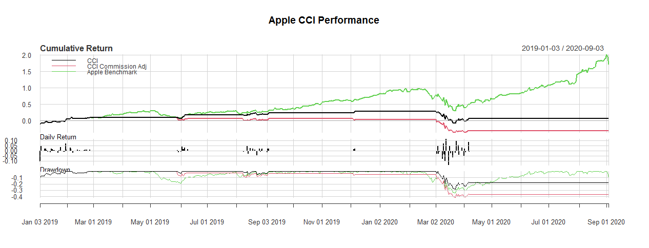

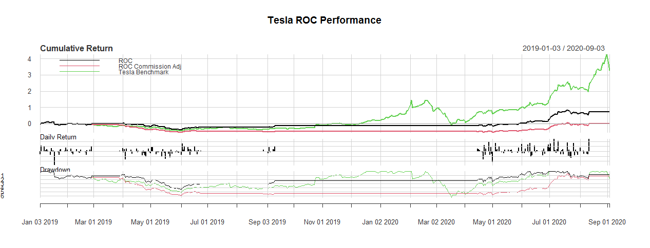
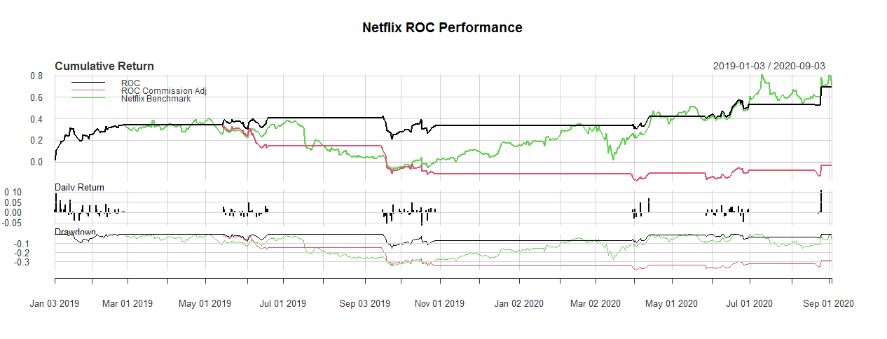
Rate Of Change (ROC)

變化率(ROC)

The following code will first calculate ROC strategy daily returns, commission adjusted ROC daily returns and finally runs the backtest (Comparison chart and an Annualized returns table) :

以下代碼將首先計算ROC策略的每日收益，傭金調整后的ROC每日收益，最后運行回溯測試(比較圖和年化收益表)：

# ROC  # 1. AAPL
roc_aapl_ret <- ret_aapl*roc_aapl_strat
roc_aapl_ret_commission_adj <- ifelse((roc_aapl_ts == 1|roc_aapl_ts == -1) & roc_aapl_strat != Lag(roc_aapl_ts), (ret_aapl-0.05)*roc_aapl_strat, ret_aapl*roc_aapl_strat)
roc_aapl_comp <- cbind(roc_aapl_ret, roc_aapl_ret_commission_adj, benchmark_aapl)
colnames(roc_aapl_comp) <- c('ROC','ROC Commission Adj','Apple Benchmark')
charts.PerformanceSummary(roc_aapl_comp, main = 'Apple ROC Performance')
roc_aapl_comp_table <- table.AnnualizedReturns(roc_aapl_comp)# 2. TSLA
roc_tsla_ret <- ret_tsla*roc_tsla_strat
roc_tsla_ret_commission_adj <- ifelse((roc_tsla_ts == 1|roc_tsla_ts == -1) & roc_tsla_strat != Lag(roc_tsla_ts), (ret_tsla-0.05)*roc_tsla_strat, ret_tsla*roc_tsla_strat)
roc_tsla_comp <- cbind(roc_tsla_ret, roc_tsla_ret_commission_adj, benchmark_tsla)
colnames(roc_tsla_comp) <- c('ROC','ROC Commission Adj','Tesla Benchmark')
charts.PerformanceSummary(roc_tsla_comp, main = 'Tesla ROC Performance')
roc_tsla_comp_table <- table.AnnualizedReturns(roc_tsla_comp)# 3. NFLX
roc_nflx_ret <- ret_nflx*roc_nflx_strat
roc_nflx_ret_commission_adj <- ifelse((roc_nflx_ts == 1|roc_nflx_ts == -1) & roc_nflx_strat != Lag(roc_nflx_ts), (ret_nflx-0.05)*roc_nflx_strat, ret_nflx*roc_nflx_strat)
roc_nflx_comp <- cbind(roc_nflx_ret, roc_nflx_ret_commission_adj, benchmark_nflx)
colnames(roc_nflx_comp) <- c('ROC','ROC Commission Adj','Netflix Benchmark')
charts.PerformanceSummary(roc_nflx_comp, main = 'Netflix ROC Performance')
roc_nflx_comp_table <- table.AnnualizedReturns(roc_nflx_comp)

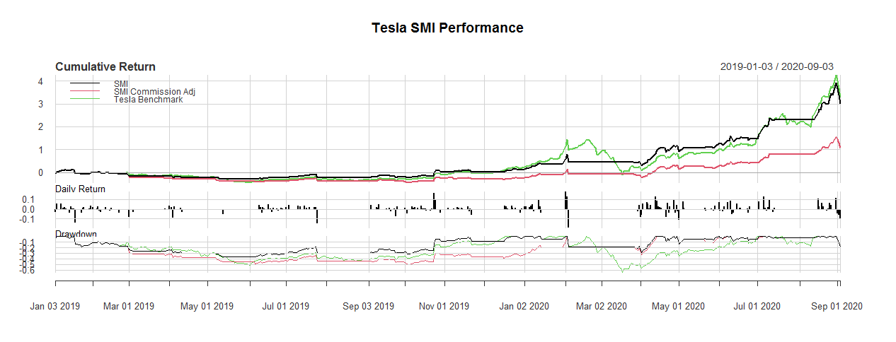
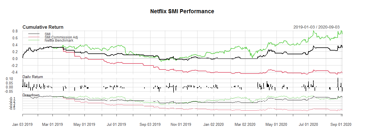
Stochastic Momentum Index (SMI)

隨機動量指數(SMI)

The following code will first calculate SMI strategy daily returns, commission adjusted SMI daily returns and finally runs the backtest (Comparison chart and an Annualized returns table) :

以下代碼將首先計算SMI策略的每日收益，傭金調整后的SMI每日收益，最后運行回溯測試(比較圖和年化收益表)：

# SMI  # 1. AAPL
smi_aapl_ret <- ret_aapl*smi_aapl_strat
smi_aapl_ret_commission_adj <- ifelse((smi_aapl_ts == 1|smi_aapl_ts == -1) & smi_aapl_strat != Lag(smi_aapl_ts), (ret_aapl-0.05)*smi_aapl_strat, ret_aapl*smi_aapl_strat)
smi_aapl_comp <- cbind(smi_aapl_ret, smi_aapl_ret_commission_adj, benchmark_aapl)
colnames(smi_aapl_comp) <- c('SMI','SMI Commission Adj','Apple Benchmark')
charts.PerformanceSummary(smi_aapl_comp, main = 'Apple SMI Performance')
smi_aapl_comp_table <- table.AnnualizedReturns(smi_aapl_comp)# 2. TSLA
smi_tsla_ret <- ret_tsla*smi_tsla_strat
smi_tsla_ret_commission_adj <- ifelse((smi_tsla_ts == 1|smi_tsla_ts == -1) & smi_tsla_strat != Lag(smi_tsla_ts), (ret_tsla-0.05)*smi_tsla_strat, ret_tsla*smi_tsla_strat)
smi_tsla_comp <- cbind(smi_tsla_ret, smi_tsla_ret_commission_adj, benchmark_tsla)
colnames(smi_tsla_comp) <- c('SMI','SMI Commission Adj','Tesla Benchmark')
charts.PerformanceSummary(smi_tsla_comp, main = 'Tesla SMI Performance')
smi_tsla_comp_table <- table.AnnualizedReturns(smi_tsla_comp)# 3. NFLX
smi_nflx_ret <- ret_nflx*smi_nflx_strat
smi_nflx_ret_commission_adj <- ifelse((smi_nflx_ts == 1|smi_nflx_ts == -1) & smi_nflx_strat != Lag(smi_nflx_ts), (ret_nflx-0.05)*smi_nflx_strat, ret_nflx*smi_nflx_strat)
smi_nflx_comp <- cbind(smi_nflx_ret, smi_nflx_ret_commission_adj, benchmark_nflx)
colnames(smi_nflx_comp) <- c('SMI','SMI Commission Adj','Netflix Benchmark')
charts.PerformanceSummary(smi_nflx_comp, main = 'Netflix SMI Performance')
smi_nflx_comp_table <- table.AnnualizedReturns(smi_nflx_comp)

Williams %R

威廉姆斯％R

The following code will first calculate Williams %R strategy daily returns, commission adjusted Williams %R daily returns and finally runs the backtest (Comparison chart and an Annualized returns table) :

以下代碼將首先計算Williams％R策略的每日收益，傭金調整后的Williams％R日收益，最后運行回溯測試(比較圖和年化收益表)：

# WPR  # 1. AAPL
wpr_aapl_ret <- ret_aapl*wpr_aapl_strat
wpr_aapl_ret_commission_adj <- ifelse((wpr_aapl_ts == 1|wpr_aapl_ts == -1) & wpr_aapl_strat != Lag(wpr_aapl_ts), (ret_aapl-0.05)*wpr_aapl_strat, ret_aapl*wpr_aapl_strat)
wpr_aapl_comp <- cbind(wpr_aapl_ret, wpr_aapl_ret_commission_adj, benchmark_aapl)
colnames(wpr_aapl_comp) <- c('WPR','WPR Commission Adj','Apple Benchmark')
charts.PerformanceSummary(wpr_aapl_comp, main = 'Apple WPR Performance')
wpr_aapl_comp_table <- table.AnnualizedReturns(wpr_aapl_comp)# 2. TSLA
wpr_tsla_ret <- ret_tsla*wpr_tsla_strat
wpr_tsla_ret_commission_adj <- ifelse((wpr_tsla_ts == 1|wpr_tsla_ts == -1) & wpr_tsla_strat != Lag(wpr_tsla_ts), (ret_tsla-0.05)*wpr_tsla_strat, ret_tsla*wpr_tsla_strat)
wpr_tsla_comp <- cbind(wpr_tsla_ret, wpr_tsla_ret_commission_adj, benchmark_tsla)
colnames(wpr_tsla_comp) <- c('WPR','WPR Commission Adj','Tesla Benchmark')
charts.PerformanceSummary(wpr_tsla_comp, main = 'Tesla WPR Performance')
wpr_tsla_comp_table <- table.AnnualizedReturns(wpr_tsla_comp)# 3. NFLX
wpr_nflx_ret <- ret_nflx*wpr_nflx_strat
wpr_nflx_ret_commission_adj <- ifelse((wpr_nflx_ts == 1|wpr_nflx_ts == -1) & wpr_nflx_strat != Lag(wpr_nflx_ts), (ret_nflx-0.05)*wpr_nflx_strat, ret_nflx*wpr_nflx_strat)
wpr_nflx_comp <- cbind(wpr_nflx_ret, wpr_nflx_ret_commission_adj, benchmark_nflx)
colnames(wpr_nflx_comp) <- c('WPR','WPR Commission Adj','Netflix Benchmark')
charts.PerformanceSummary(wpr_nflx_comp, main = 'Netflix WPR Performance')
wpr_nflx_comp_table <- table.AnnualizedReturns(wpr_nflx_comp)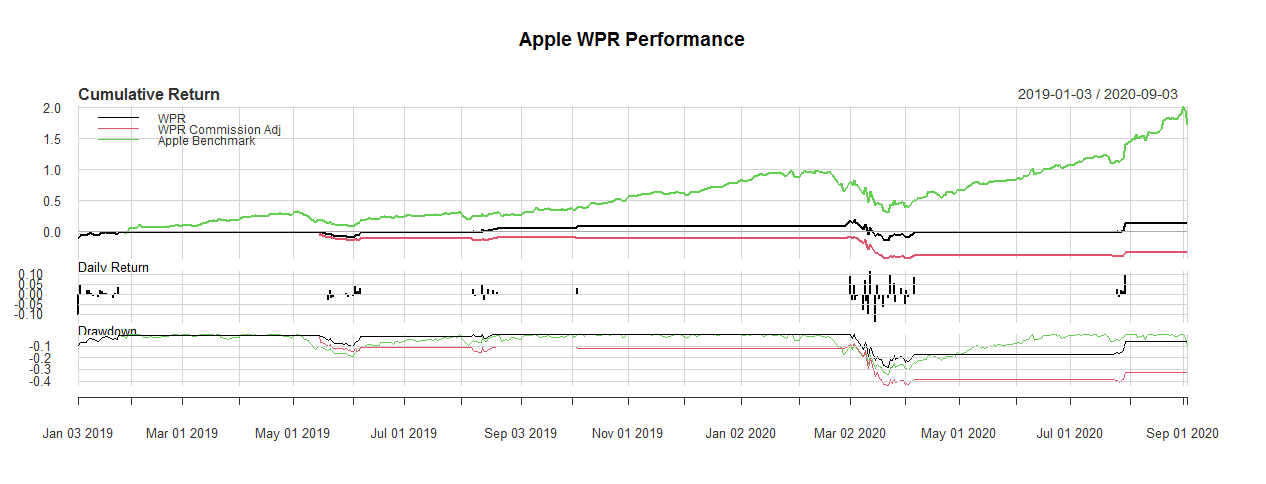

最后的想法！ (Final Thoughts!)

Hurrah! We successfully finished our process of creating trading strategies and backtesting the results with R. I want to highlight that, every strategies and backtesting results are only for educational purpose and should not be taken as an investment advice. Apart from our created strategies, you can do your coding and frame your own trading strategies based on our needs and flexibility. If you’ve missed any of the coding sections, no worries. I’ve added the full code file at the end. In this article, we’ve covered only six major technical indicators but, there are more to discover. So, never stop learning and never stop coding!

歡呼！ 我們成功地完成了創建交易策略并使用R對結果進行回測的過程。我想強調一點，每一種策略和回測結果僅用于教育目的，不應被視為投資建議。 除了我們創建的策略之外，您還可以根據我們的需求和靈活性進行編碼并制定自己的交易策略。 如果您錯過了任何編碼部分，請不要擔心。 我在末尾添加了完整的代碼文件。 在本文中，我們僅介紹了六個主要技術指標，但還有更多發現之處。 因此，永遠不要停止學習，永遠不要停止編碼！

Happy Coding and Analyzing!

快樂的編碼和分析！

Full Code :

完整代碼：

library(quantmod)
library(TTR)
library(PerformanceAnalytics)# Getting stock prices of AAPL, TSLA and NFLX
getSymbols('AAPL', src = 'yahoo', from = '2019-01-01')
getSymbols('TSLA', src = 'yahoo', from = '2019-01-01')
getSymbols('NFLX', src = 'yahoo', from = '2019-01-01')# Basic plot of the three stocks
barChart(AAPL, theme = chartTheme('black'))
barChart(TSLA, theme = chartTheme('black'))
barChart(NFLX, theme = chartTheme('black'))# Creating Leading and Lagging Technical Indicators# a. Simple Moving Average (SMA)# 1. AAPL
sma20_aapl <- SMA(AAPL$AAPL.Close, n = 20)
sma50_aapl <- SMA(AAPL$AAPL.Close, n = 50)
lineChart(AAPL, theme = chartTheme('black'))
addSMA(n = 20, col = 'blue')
addSMA(n = 50, col = 'orange')
legend('left', col = c('green','blue','orange'),legend = c('AAPL','SMA20','SMA50'), lty = 1, bty = 'n',text.col = 'white', cex = 0.8)
# 2. TSLA
sma20_tsla <- SMA(TSLA$TSLA.Close, n = 20)
sma50_tsla <- SMA(TSLA$TSLA.Close, n = 50)
lineChart(TSLA, theme = 'black')
addSMA(n = 20, col = 'blue')
addSMA(n = 50, col = 'orange')
legend('left', col = c('green','blue','orange'),legend = c('AAPL','SMA20','SMA50'), lty = 1, bty = 'n',text.col = 'white', cex = 0.8)
# 3. NFLX
sma20_nflx <- SMA(NFLX$NFLX.Close, n = 20)
sma50_nflx <- SMA(NFLX$NFLX.Close, n = 50)
lineChart(NFLX, theme = 'black')
addSMA(n = 20, col = 'blue')
addSMA(n = 50, col = 'orange')
legend('left', col = c('green','blue','orange'),legend = c('AAPL','SMA20','SMA50'), lty = 1, bty = 'n',text.col = 'white', cex = 0.8)# b.  Parabolic Stop And Reverse (SAR)# 1. AAPL
sar_aapl <- SAR(cbind(Hi(AAPL),Lo(AAPL)), accel = c(0.02, 0.2))
barChart(AAPL, theme = 'black')
addSAR(accel = c(0.02, 0.2), col = 'lightblue')
# 2. TSLA
sar_tsla <- SAR(cbind(Hi(TSLA),Lo(TSLA)), accel = c(0.02, 0.2))
barChart(TSLA, theme = 'black')
addSAR(accel = c(0.02, 0.2), col = 'lightblue')
# 3. NFLX
sar_nflx <- SAR(cbind(Hi(NFLX),Lo(NFLX)), accel = c(0.02, 0.2))
barChart(NFLX, theme = 'black')
addSAR(accel = c(0.02, 0.2), col = 'lightblue')# c. Commodity Channel Index (CCI)# 1. AAPL
cci_aapl <- CCI(HLC(AAPL), n = 20, c = 0.015)
barChart(AAPL, theme = 'black')
addCCI(n = 20, c = 0.015)
# 2. TSLA
cci_tsla <- CCI(HLC(TSLA), n = 20, c = 0.015)
barChart(TSLA, theme = 'black')
addCCI(n = 20, c = 0.015)
# 3. NFLX
cci_nflx <- CCI(HLC(NFLX), n = 20, c = 0.015)
barChart(NFLX, theme = 'black')
addCCI(n = 20, c = 0.015)# d. Rate of Change (ROC)# 1. AAPL
roc_aapl <- ROC(AAPL$AAPL.Close, n = 25)
barChart(AAPL, theme = 'black')
addROC(n = 25)
legend('left', col = 'red', legend = 'ROC(25)', lty = 1, bty = 'n',text.col = 'white', cex = 0.8)
# 1. TSLA
roc_tsla <- ROC(TSLA$TSLA.Close, n = 25)
barChart(TSLA, theme = 'black')
addROC(n = 25)
legend('left', col = 'red', legend = 'ROC(25)', lty = 1, bty = 'n',text.col = 'white', cex = 0.8)
# 1. NFLX
roc_nflx <- ROC(NFLX$NFLX.Close, n = 25)
barChart(NFLX, theme = 'black')
addROC(n = 25)
legend('right', col = 'red', legend = 'ROC(25)', lty = 1, bty = 'n',text.col = 'white', cex = 0.8)# e. Stochastic Momentum Index (SMI)# 1. AAPL
smi_aapl <- SMI(HLC(AAPL),n = 13, nFast = 2, nSlow = 25, nSig = 9)
barChart(AAPL, theme = 'black')
addSMI(n = 13, fast = 2, slow = 2, signal = 9)
# 2. TSLA
smi_tsla <- SMI(HLC(TSLA),n = 13, nFast = 2, nSlow = 25, nSig = 9)
barChart(TSLA, theme = 'black')
addSMI(n = 13, fast = 2, slow = 2, signal = 9)
# 3. NFLX
smi_nflx <- SMI(HLC(NFLX),n = 13, nFast = 2, nSlow = 25, nSig = 9)
barChart(NFLX, theme = 'black')
addSMI(n = 13, fast = 2, slow = 2, signal = 9)# f. Williams %R# 1. AAPL
wpr_aapl <- WPR(HLC(AAPL), n = 14)
colnames(wpr_aapl) <- 'wpr'
barChart(AAPL, theme = 'black')
addWPR(n = 14)
# 1. TSLA
wpr_tsla <- WPR(HLC(TSLA), n = 14)
colnames(wpr_tsla) <- 'wpr'
barChart(TSLA, theme = 'black')
addWPR(n = 14)
# 1. NFLX
wpr_nflx <- WPR(HLC(NFLX), n = 14)
colnames(wpr_nflx) <- 'wpr'
barChart(NFLX, theme = 'black')
addWPR(n = 14)# Creating Trading signal with Indicators# SMA # a. AAPL
# SMA 20 Crossover Signal 
sma20_aapl_ts <- Lag(ifelse(Lag(Cl(AAPL)) < Lag(sma20_aapl) & Cl(AAPL) > sma20_aapl,1,ifelse(Lag(Cl(AAPL)) > Lag(sma20_aapl) & Cl(AAPL) < sma20_aapl,-1,0)))
sma20_aapl_ts[is.na(sma20_aapl_ts)] <- 0
# SMA 50 Crossover Signal
sma50_aapl_ts <- Lag(ifelse(Lag(Cl(AAPL)) < Lag(sma50_aapl) & Cl(AAPL) > sma50_aapl,1,ifelse(Lag(Cl(AAPL)) > Lag(sma50_aapl) & Cl(AAPL) < sma50_aapl,-1,0)))
sma50_aapl_ts[is.na(sma50_aapl_ts)] <- 0
# SMA 20 and SMA 50 Crossover Signal
sma_aapl_ts <- Lag(ifelse(Lag(sma20_aapl) < Lag(sma50_aapl) & sma20_aapl > sma50_aapl,1,ifelse(Lag(sma20_aapl) > Lag(sma50_aapl) & sma20_aapl < sma50_aapl,-1,0)))
sma_aapl_ts[is.na(sma_aapl_ts)] <- 0# b. TSLA
# SMA 20 Crossover Signal 
sma20_tsla_ts <- Lag(ifelse(Lag(Cl(TSLA)) < Lag(sma20_tsla) & Cl(TSLA) > sma20_tsla,1,ifelse(Lag(Cl(TSLA)) > Lag(sma20_tsla) & Cl(TSLA) < sma20_tsla,-1,0)))
sma20_tsla_ts[is.na(sma20_tsla_ts)] <- 0
# SMA 50 Crossover Signal
sma50_tsla_ts <- Lag(ifelse(Lag(Cl(TSLA)) < Lag(sma50_tsla) & Cl(TSLA) > sma50_tsla,1,ifelse(Lag(Cl(TSLA)) > Lag(sma50_tsla) & Cl(TSLA) < sma50_tsla,-1,0)))
sma50_tsla_ts[is.na(sma50_tsla_ts)] <- 0
# SMA 20 and SMA 50 Crossover Signal
sma_tsla_ts <- Lag(ifelse(Lag(sma20_tsla) < Lag(sma50_tsla) & sma20_tsla > sma50_tsla,1,ifelse(Lag(sma20_tsla) > Lag(sma50_tsla) & sma20_tsla < sma50_tsla,-1,0)))
sma_tsla_ts[is.na(sma_tsla_ts)] <- 0# c. NFLX
# SMA 20 Crossover Signal 
sma20_nflx_ts <- Lag(ifelse(Lag(Cl(NFLX)) < Lag(sma20_nflx) & Cl(NFLX) > sma20_nflx,1,ifelse(Lag(Cl(NFLX)) > Lag(sma20_nflx) & Cl(NFLX) < sma20_nflx,-1,0)))
sma20_nflx_ts[is.na(sma20_nflx_ts)] <- 0
# SMA 50 Crossover Signal
sma50_nflx_ts <- Lag(ifelse(Lag(Cl(NFLX)) < Lag(sma50_nflx) & Cl(NFLX) > sma50_nflx,1,ifelse(Lag(Cl(NFLX)) > Lag(sma50_nflx) & Cl(NFLX) < sma50_nflx,-1,0)))
sma50_nflx_ts[is.na(sma50_nflx_ts)] <- 0
# SMA 20 and SMA 50 Crossover Signal
sma_nflx_ts <- Lag(ifelse(Lag(sma20_nflx) < Lag(sma50_nflx) & sma20_nflx > sma50_nflx,1,ifelse(Lag(sma20_nflx) > Lag(sma50_nflx) & sma20_nflx < sma50_nflx,-1,0)))
sma_nflx_ts[is.na(sma_nflx_ts)] <- 0# 2. Parabolic Stop And Reverse (SAR) # a. AAPL
sar_aapl_ts <- Lag(ifelse(Lag(Cl(AAPL)) < Lag(sar_aapl) & Cl(AAPL) > sar_aapl,1,ifelse(Lag(Cl(AAPL)) > Lag(sar_aapl) & Cl(AAPL) < sar_aapl,-1,0)))
sar_aapl_ts[is.na(sar_aapl_ts)] <- 0
# b. TSLA
sar_tsla_ts <- Lag(ifelse(Lag(Cl(TSLA)) < Lag(sar_tsla) & Cl(TSLA) > sar_tsla,1,ifelse(Lag(Cl(TSLA)) > Lag(sar_tsla) & Cl(TSLA) < sar_tsla,-1,0)))
sar_tsla_ts[is.na(sar_tsla_ts)] <- 0
# c. NFLX
sar_nflx_ts <- Lag(ifelse(Lag(Cl(NFLX)) < Lag(sar_nflx) & Cl(NFLX) > sar_nflx,1,ifelse(Lag(Cl(NFLX)) > Lag(sar_nflx) & Cl(NFLX) < sar_nflx,-1,0)))
sar_nflx_ts[is.na(sar_nflx_ts)] <- 0# 3. Commodity Channel Index  (CCI)# a. AAPL
cci_aapl_ts <- Lag(ifelse(Lag(cci_aapl) < (-100) & cci_aapl > (-100),1,ifelse(Lag(cci_aapl) < (100) & cci_aapl > (100),-1,0)))
cci_aapl_ts[is.na(cci_aapl_ts)] <- 0
# b. TSLA
cci_tsla_ts <- Lag(ifelse(Lag(cci_tsla) < (-100) & cci_tsla > (-100),1,ifelse(Lag(cci_tsla) < (100) & cci_tsla > (100),-1,0)))
cci_tsla_ts[is.na(cci_tsla_ts)] <- 0
# c. NFLX
cci_nflx_ts <- Lag(ifelse(Lag(cci_nflx) < (-100) & cci_nflx > (-100),1,ifelse(Lag(cci_nflx) < (100) & cci_nflx > (100),-1,0)))
cci_nflx_ts[is.na(cci_nflx_ts)] <- 0# 4. Rate of Change (ROC)# a. AAPL
roc_aapl_ts <- Lag(ifelse(Lag(roc_aapl) < (-0.05) & roc_aapl > (-0.05),1,ifelse(Lag(roc_aapl) < (0.05) & roc_aapl > (0.05),-1,0)))
roc_aapl_ts[is.na(roc_aapl_ts)] <- 0
# b. TSLA
roc_tsla_ts <- Lag(ifelse(Lag(roc_tsla) < (-0.05) & roc_tsla > (-0.05),1,ifelse(Lag(roc_tsla) < (0.05) & roc_tsla > (0.05),-1,0)))
roc_tsla_ts[is.na(roc_tsla_ts)] <- 0
# c. NFLX
roc_nflx_ts <- Lag(ifelse(Lag(roc_nflx) < (-0.05) & roc_nflx > (-0.05),1,ifelse(Lag(roc_nflx) < (0.05) & roc_nflx > (0.05),-1,0)))
roc_nflx_ts[is.na(roc_nflx_ts)] <- 0# 5. Stochastic Momentum Index (SMI)# a. AAPL
smi_aapl_ts <- Lag(ifelse(Lag(smi_aapl[,1]) < Lag(smi_aapl[,2]) & smi_aapl[,1] > smi_aapl[,2],1, ifelse(Lag(smi_aapl[,1]) > Lag(smi_aapl[,2]) & smi_aapl[,1] < smi_aapl[,2],-1,0)))
smi_aapl_ts[is.na(smi_aapl_ts)] <- 0
# b. TSLA
smi_tsla_ts <- Lag(ifelse(Lag(smi_tsla[,1]) < Lag(smi_tsla[,2]) & smi_tsla[,1] > smi_tsla[,2],1, ifelse(Lag(smi_tsla[,1]) > Lag(smi_tsla[,2]) & smi_tsla[,1] < smi_tsla[,2],-1,0)))
smi_tsla_ts[is.na(smi_tsla_ts)] <- 0
# a. NFLX
smi_nflx_ts <- Lag(ifelse(Lag(smi_nflx[,1]) < Lag(smi_nflx[,2]) & smi_nflx[,1] > smi_nflx[,2],1, ifelse(Lag(smi_nflx[,1]) > Lag(smi_nflx[,2]) & smi_nflx[,1] < smi_nflx[,2],-1,0)))
smi_nflx_ts[is.na(smi_nflx_ts)] <- 0# 6. williams %R# a. AAPL
wpr_aapl_ts <- Lag(ifelse(Lag(wpr_aapl) > 0.8 & wpr_aapl < 0.8,1,ifelse(Lag(wpr_aapl) > 0.2 & wpr_aapl < 0.2,-1,0)))
wpr_aapl_ts[is.na(wpr_aapl_ts)] <- 0
# b. TSLA
wpr_tsla_ts <- Lag(ifelse(Lag(wpr_tsla) > 0.8 & wpr_tsla < 0.8,1,ifelse(Lag(wpr_tsla) > 0.2 & wpr_tsla < 0.2,-1,0)))
wpr_tsla_ts[is.na(wpr_tsla_ts)] <- 0
# c. NFLX
wpr_nflx_ts <- Lag(ifelse(Lag(wpr_nflx) > 0.8 & wpr_nflx < 0.8,1,ifelse(Lag(wpr_nflx) > 0.2 & wpr_nflx < 0.2,-1,0)))
wpr_nflx_ts[is.na(wpr_nflx_ts)] <- 0# Creating Trading Strategies using Signals# 1. SMA 20 and SMA 50 Crossover Strategy# a. AAPL
sma_aapl_strat <- ifelse(sma_aapl_ts > 1,0,1)
for (i in 1 : length(Cl(AAPL))) {sma_aapl_strat[i] <- ifelse(sma_aapl_ts[i] == 1,1,ifelse(sma_aapl_ts[i] == -1,0,sma_aapl_strat[i-1]))
}
sma_aapl_strat[is.na(sma_aapl_strat)] <- 1
sma_aapl_stratcomp <- cbind(sma20_aapl, sma50_aapl, sma_aapl_ts, sma_aapl_strat)
colnames(sma_aapl_stratcomp) <- c('SMA(20)','SMA(50)','SMA SIGNAL','SMA POSITION')
# b. TSLA
sma_tsla_strat <- ifelse(sma_tsla_ts > 1,0,1)
for (i in 1 : length(Cl(TSLA))) {sma_tsla_strat[i] <- ifelse(sma_tsla_ts[i] == 1,1,ifelse(sma_tsla_ts[i] == -1,0,sma_tsla_strat[i-1]))
}
sma_tsla_strat[is.na(sma_tsla_strat)] <- 1
sma_tsla_stratcomp <- cbind(sma20_tsla, sma50_tsla, sma_tsla_ts, sma_tsla_strat)
colnames(sma_tsla_stratcomp) <- c('SMA(20)','SMA(50)','SMA SIGNAL','SMA POSITION')
# c. NFLX
sma_nflx_strat <- ifelse(sma_nflx_ts > 1,0,1)
for (i in 1 : length(Cl(NFLX))) {sma_nflx_strat[i] <- ifelse(sma_nflx_ts[i] == 1,1,ifelse(sma_nflx_ts[i] == 'SEL',0,sma_nflx_strat[i-1]))
}
sma_nflx_strat[is.na(sma_nflx_strat)] <- 1
sma_nflx_stratcomp <- cbind(sma20_nflx, sma50_nflx, sma_nflx_ts, sma_nflx_strat)
colnames(sma_nflx_stratcomp) <- c('SMA(20)','SMA(50)','SMA SIGNAL','SMA POSITION')# Parabolic SAR Strategy # a. AAPL
sar_aapl_strat <- ifelse(sar_aapl_ts > 1,0,1)
for (i in 1 : length(Cl(AAPL))) {sar_aapl_strat[i] <- ifelse(sar_aapl_ts[i] == 1,1,ifelse(sar_aapl_ts[i] == -1,0,sar_aapl_strat[i-1]))
}
sar_aapl_strat[is.na(sar_aapl_strat)] <- 1
sar_aapl_stratcomp <- cbind(Cl(AAPL), sar_aapl, sar_aapl_ts, sar_aapl_strat)
colnames(sar_aapl_stratcomp) <- c('Close','SAR','SAR SIGNAL','SAR POSITION')
# b. TSLA
sar_tsla_strat <- ifelse(sar_tsla_ts > 1,0,1)
for (i in 1 : length(Cl(TSLA))) {sar_tsla_strat[i] <- ifelse(sar_tsla_ts[i] == 1,1,ifelse(sar_tsla_ts[i] == -1,0,sar_tsla_strat[i-1]))
}
sar_tsla_strat[is.na(sar_tsla_strat)] <- 1
sar_tsla_stratcomp <- cbind(Cl(TSLA), sar_tsla, sar_tsla_ts, sar_tsla_strat)
colnames(sar_tsla_stratcomp) <- c('Close','SAR','SAR SIGNAL','SAR POSITION')
# c. NFLX
sar_nflx_strat <- ifelse(sar_nflx_ts > 1,0,1)
for (i in 1 : length(Cl(NFLX))) {sar_nflx_strat[i] <- ifelse(sar_nflx_ts[i] == 1,1,ifelse(sar_nflx_ts[i] == -1,0,sar_nflx_strat[i-1]))
}
sar_nflx_strat[is.na(sar_nflx_strat)] <- 1
sar_nflx_stratcomp <- cbind(Cl(NFLX), sar_nflx, sar_nflx_ts, sar_nflx_strat)
colnames(sar_nflx_stratcomp) <- c('Close','SAR','SAR SIGNAL','SAR POSITION')# CCI# a. AAPL
cci_aapl_strat <- ifelse(cci_aapl_ts > 1,0,1)
for (i in 1 : length(Cl(AAPL))) {cci_aapl_strat[i] <- ifelse(cci_aapl_ts[i] == 1,1,ifelse(cci_aapl_ts[i] == -1,0,cci_aapl_strat[i-1]))
}
cci_aapl_strat[is.na(cci_aapl_strat)] <- 1
cci_aapl_stratcomp <- cbind(cci_aapl, cci_aapl_ts, cci_aapl_strat)
colnames(cci_aapl_stratcomp) <- c('CCI','CCI SIGNAL','CCI POSITION')
# b. TSLA
cci_tsla_strat <- ifelse(cci_tsla_ts > 1,0,1)
for (i in 1 : length(Cl(TSLA))) {cci_tsla_strat[i] <- ifelse(cci_tsla_ts[i] == 1,1,ifelse(cci_tsla_ts[i] == -1,0,cci_tsla_strat[i-1]))
}
cci_tsla_strat[is.na(cci_tsla_strat)] <- 1
cci_tsla_stratcomp <- cbind(cci_tsla, cci_tsla_ts, cci_tsla_strat)
colnames(cci_tsla_stratcomp) <- c('CCI','CCI SIGNAL','CCI POSITION')
# c. NFLX
cci_nflx_strat <- ifelse(cci_nflx_ts > 1,0,1)
for (i in 1 : length(Cl(NFLX))) {cci_nflx_strat[i] <- ifelse(cci_nflx_ts[i] == 1,1,ifelse(cci_nflx_ts[i] == -1,0,cci_nflx_strat[i-1]))
}
cci_nflx_strat[is.na(cci_nflx_strat)] <- 1
cci_nflx_stratcomp <- cbind(cci_nflx, cci_nflx_ts, cci_nflx_strat)
colnames(cci_nflx_stratcomp) <- c('CCI','CCI SIGNAL','CCI POSITION')# ROC# a. AAPL
roc_aapl_strat <- ifelse(roc_aapl_ts > 1,0,1)
for (i in 1 : length(Cl(AAPL))) {roc_aapl_strat[i] <- ifelse(roc_aapl_ts[i] == 1,1,ifelse(roc_aapl_ts[i] == -1,0,roc_aapl_strat[i-1]))
}
roc_aapl_strat[is.na(roc_aapl_strat)] <- 1
roc_aapl_stratcomp <- cbind(roc_aapl, roc_aapl_ts, roc_aapl_strat)
colnames(roc_aapl_stratcomp) <- c('ROC(25)','ROC SIGNAL','ROC POSITION')
# b. TSLA
roc_tsla_strat <- ifelse(roc_tsla_ts > 1,0,1)
for (i in 1 : length(Cl(TSLA))) {roc_tsla_strat[i] <- ifelse(roc_tsla_ts[i] == 1,1,ifelse(roc_tsla_ts[i] == -1,0,roc_tsla_strat[i-1]))
}
roc_tsla_strat[is.na(roc_tsla_strat)] <- 1
roc_tsla_stratcomp <- cbind(roc_tsla, roc_tsla_ts, roc_tsla_strat)
colnames(roc_tsla_stratcomp) <- c('ROC(25)','ROC SIGNAL','ROC POSITION')
# c. NFLX
roc_nflx_strat <- ifelse(roc_nflx_ts > 1,0,1)
for (i in 1 : length(Cl(NFLX))) {roc_nflx_strat[i] <- ifelse(roc_nflx_ts[i] == 1,1,ifelse(roc_nflx_ts[i] == -1,0,roc_nflx_strat[i-1]))
}
roc_nflx_strat[is.na(roc_nflx_strat)] <- 1
roc_nflx_stratcomp <- cbind(roc_nflx, roc_nflx_ts, roc_nflx_strat)
colnames(roc_nflx_stratcomp) <- c('ROC(25)','ROC SIGNAL','ROC POSITION')# SMI# a. AAPL
smi_aapl_strat <- ifelse(smi_aapl_ts > 1,0,1)
for (i in 1 : length(Cl(AAPL))) {smi_aapl_strat[i] <- ifelse(smi_aapl_ts[i] == 1,1,ifelse(smi_aapl_ts[i] == -1,0,smi_aapl_strat[i-1]))
}
smi_aapl_strat[is.na(smi_aapl_strat)] <- 1
smi_aapl_stratcomp <- cbind(smi_aapl[,1],smi_aapl[,2],smi_aapl_ts,smi_aapl_strat)
colnames(smi_aapl_stratcomp) <- c('SMI','SMI(S)','SMI SIGNAL','SMI POSITION')
# b. TSLA
smi_tsla_strat <- ifelse(smi_tsla_ts > 1,0,1)
for (i in 1 : length(Cl(TSLA))) {smi_tsla_strat[i] <- ifelse(smi_tsla_ts[i] == 1,1,ifelse(smi_tsla_ts[i] == -1,0,smi_tsla_strat[i-1]))
}
smi_tsla_strat[is.na(smi_tsla_strat)] <- 1
smi_tsla_stratcomp <- cbind(smi_tsla[,1],smi_tsla[,2],smi_tsla_ts,smi_tsla_strat)
colnames(smi_tsla_stratcomp) <- c('SMI','SMI(S)','SMI SIGNAL','SMI POSITION')
# c. NFLX
smi_nflx_strat <- ifelse(smi_nflx_ts > 1,0,1)
for (i in 1 : length(Cl(NFLX))) {smi_nflx_strat[i] <- ifelse(smi_nflx_ts[i] == 1,1,ifelse(smi_nflx_ts[i] == -1,0,smi_nflx_strat[i-1]))
}
smi_nflx_strat[is.na(smi_nflx_strat)] <- 1
smi_nflx_stratcomp <- cbind(smi_nflx[,1],smi_nflx[,2],smi_nflx_ts,smi_nflx_strat)
colnames(smi_nflx_stratcomp) <- c('SMI','SMI(S)','SMI SIGNAL','SMI POSITION')# WPR# a. AAPL
wpr_aapl_strat <- ifelse(wpr_aapl_ts > 1,0,1)
for (i in 1 : length(Cl(AAPL))) {wpr_aapl_strat[i] <- ifelse(wpr_aapl_ts[i] == 1,1,ifelse(wpr_aapl_ts[i] == -1,0,wpr_aapl_strat[i-1]))
}
wpr_aapl_strat[is.na(wpr_aapl_strat)] <- 1
wpr_aapl_stratcomp <- cbind(wpr_aapl, wpr_aapl_ts, wpr_aapl_strat)
colnames(wpr_aapl_stratcomp) <- c('WPR(14)','WPR SIGNAL','WPR POSITION')
# b. TSLA
wpr_tsla_strat <- ifelse(wpr_tsla_ts > 1,0,1)
for (i in 1 : length(Cl(TSLA))) {wpr_tsla_strat[i] <- ifelse(wpr_tsla_ts[i] == 1,1,ifelse(wpr_tsla_ts[i] == -1,0,wpr_tsla_strat[i-1]))
}
wpr_tsla_strat[is.na(wpr_tsla_strat)] <- 1
wpr_tsla_stratcomp <- cbind(wpr_tsla, wpr_tsla_ts, wpr_tsla_strat)
colnames(wpr_tsla_stratcomp) <- c('WPR(14)','WPR SIGNAL','WPR POSITION')
# c. NFLX
wpr_nflx_strat <- ifelse(wpr_nflx_ts > 1,0,1)
for (i in 1 : length(Cl(NFLX))) {wpr_nflx_strat[i] <- ifelse(wpr_nflx_ts[i] == 1,1,ifelse(wpr_nflx_ts[i] == -1,0,wpr_nflx_strat[i-1]))
}
wpr_nflx_strat[is.na(wpr_nflx_strat)] <- 1
wpr_nflx_stratcomp <- cbind(wpr_nflx, wpr_nflx_ts, wpr_nflx_strat)
colnames(wpr_nflx_stratcomp) <- c('WPR(14)','WPR SIGNAL','WPR POSITION')# Trading Strategy Performance # Calculating Returns & setting Benchmark for companies
ret_aapl <- diff(log(Cl(AAPL)))
ret_tsla <- diff(log(Cl(TSLA)))
ret_nflx <- diff(log(Cl(NFLX)))
benchmark_aapl <- ret_aapl
benchmark_tsla <- ret_tsla
benchmark_nflx <- ret_nflx# SMA # 1. AAPL
sma_aapl_ret <- ret_aapl*sma_aapl_strat
sma_aapl_ret_commission_adj <- ifelse((sma_aapl_ts == 1|sma_aapl_ts == -1) & sma_aapl_strat != Lag(sma_aapl_ts), (ret_aapl-0.05)*sma_aapl_strat, ret_aapl*sma_aapl_strat)
sma_aapl_comp <- cbind(sma_aapl_ret, sma_aapl_ret_commission_adj, benchmark_aapl)
colnames(sma_aapl_comp) <- c('SMA','SMA Commission Adj','Apple Benchmark')
charts.PerformanceSummary(sma_aapl_comp, main = 'Apple SMA Performance')
sma_aapl_comp_table <- table.AnnualizedReturns(sma_aapl_comp)
# 2. TSLA
sma_tsla_ret <- ret_tsla*sma_tsla_strat
sma_tsla_ret_commission_adj <- ifelse((sma_tsla_ts == 1|sma_tsla_ts == -1) & sma_tsla_strat != Lag(sma_tsla_ts), (ret_tsla-0.05)*sma_tsla_strat, ret_tsla*sma_tsla_strat)
sma_tsla_comp <- cbind(sma_tsla_ret, sma_tsla_ret_commission_adj, benchmark_tsla)
colnames(sma_tsla_comp) <- c('SMA','SMA Commission Adj','Tesla Benchmark')
charts.PerformanceSummary(sma_tsla_comp, main = 'Tesla SMA Performance')
sma_tsla_comp_table <- table.AnnualizedReturns(sma_tsla_comp)
# 3. NFLX
sma_nflx_ret <- ret_nflx*sma_nflx_strat
sma_nflx_ret_commission_adj <- ifelse((sma_nflx_ts == 1|sma_nflx_ts == -1) & sma_nflx_strat != Lag(sma_nflx_ts), (ret_nflx-0.05)*sma_nflx_strat, ret_nflx*sma_nflx_strat)
sma_nflx_comp <- cbind(sma_nflx_ret, sma_nflx_ret_commission_adj, benchmark_nflx)
colnames(sma_nflx_comp) <- c('SMA','SMA Commission Adj','Netflix Benchmark')
charts.PerformanceSummary(sma_nflx_comp, main = 'Netflix SMA Performance')
sma_nflx_comp_table <- table.AnnualizedReturns(sma_nflx_comp)# Parabolic SAR # 1. AAPL
sar_aapl_ret <- ret_aapl*sar_aapl_strat
sar_aapl_ret_commission_adj <- ifelse((sar_aapl_ts == 1|sar_aapl_ts == -1) & sar_aapl_strat != Lag(sar_aapl_ts), (ret_aapl-0.05)*sar_aapl_strat, ret_aapl*sar_aapl_strat)
sar_aapl_comp <- cbind(sar_aapl_ret, sar_aapl_ret_commission_adj, benchmark_aapl)
colnames(sar_aapl_comp) <- c('SAR','SAR Commission Adj','Apple Benchmark')
charts.PerformanceSummary(sar_aapl_comp, main = 'Apple Parabolic SAR Performance')
sar_aapl_comp_table <- table.AnnualizedReturns(sar_aapl_comp)
# 2. TSLA
sar_tsla_ret <- ret_tsla*sar_tsla_strat
sar_tsla_ret_commission_adj <- ifelse((sar_tsla_ts == 1|sar_tsla_ts == -1) & sar_tsla_strat != Lag(sar_tsla_ts), (ret_tsla-0.05)*sar_tsla_strat, ret_tsla*sar_tsla_strat)
sar_tsla_comp <- cbind(sar_tsla_ret, sar_tsla_ret_commission_adj, benchmark_tsla)
colnames(sar_tsla_comp) <- c('SAR','SAR Commission Adj','Tesla Benchmark')
charts.PerformanceSummary(sar_tsla_comp, main = 'Tesla Parabolic SAR Performance')
sar_tsla_comp_table <- table.AnnualizedReturns(sar_tsla_comp)
# 3. NFLX
sar_nflx_ret <- ret_nflx*sar_nflx_strat
sar_nflx_ret_commission_adj <- ifelse((sar_nflx_ts == 1|sar_nflx_ts == -1) & sar_nflx_strat != Lag(sar_nflx_ts), (ret_nflx-0.05)*sar_nflx_strat, ret_nflx*sar_nflx_strat)
sar_nflx_comp <- cbind(sar_nflx_ret, sar_nflx_ret_commission_adj, benchmark_nflx)
colnames(sar_nflx_comp) <- c('SAR','SAR Commission Adj','Netflix Benchmark')
charts.PerformanceSummary(sar_nflx_comp, main = 'Netflix Parabolic SAR Performance')
sar_nflx_comp_table <- table.AnnualizedReturns(sar_nflx_comp)# CCI  # 1. AAPL
cci_aapl_ret <- ret_aapl*cci_aapl_strat
cci_aapl_ret_commission_adj <- ifelse((cci_aapl_ts == 1|cci_aapl_ts == -1) & cci_aapl_strat != Lag(cci_aapl_ts), (ret_aapl-0.05)*cci_aapl_strat, ret_aapl*cci_aapl_strat)
cci_aapl_comp <- cbind(cci_aapl_ret, cci_aapl_ret_commission_adj, benchmark_aapl)
colnames(cci_aapl_comp) <- c('CCI','CCI Commission Adj','Apple Benchmark')
charts.PerformanceSummary(cci_aapl_comp, main = 'Apple CCI Performance')
cci_aapl_comp_table <- table.AnnualizedReturns(cci_aapl_comp)
# 2. TSLA
cci_tsla_ret <- ret_tsla*cci_tsla_strat
cci_tsla_ret_commission_adj <- ifelse((cci_tsla_ts == 1|cci_tsla_ts == -1) & cci_tsla_strat != Lag(cci_tsla_ts), (ret_tsla-0.05)*cci_tsla_strat, ret_tsla*cci_tsla_strat)
cci_tsla_comp <- cbind(cci_tsla_ret, cci_tsla_ret_commission_adj, benchmark_tsla)
colnames(cci_tsla_comp) <- c('CCI','CCI Commission Adj','Tesla Benchmark')
charts.PerformanceSummary(cci_tsla_comp, main = 'Tesla CCI Performance')
cci_tsla_comp_table <- table.AnnualizedReturns(cci_tsla_comp)
# 3. NFLX
cci_nflx_ret <- ret_nflx*cci_nflx_strat
cci_nflx_ret_commission_adj <- ifelse((cci_nflx_ts == 1|cci_nflx_ts == -1) & cci_nflx_strat != Lag(cci_nflx_ts), (ret_nflx-0.05)*cci_nflx_strat, ret_nflx*cci_nflx_strat)
cci_nflx_comp <- cbind(cci_nflx_ret, cci_nflx_ret_commission_adj, benchmark_nflx)
colnames(cci_nflx_comp) <- c('CCI','CCI Commission Adj','Netflix Benchmark')
charts.PerformanceSummary(cci_nflx_comp, main = 'Netflix CCI Performance')
cci_nflx_comp_table <- table.AnnualizedReturns(cci_nflx_comp)# ROC  # 1. AAPL
roc_aapl_ret <- ret_aapl*roc_aapl_strat
roc_aapl_ret_commission_adj <- ifelse((roc_aapl_ts == 1|roc_aapl_ts == -1) & roc_aapl_strat != Lag(roc_aapl_ts), (ret_aapl-0.05)*roc_aapl_strat, ret_aapl*roc_aapl_strat)
roc_aapl_comp <- cbind(roc_aapl_ret, roc_aapl_ret_commission_adj, benchmark_aapl)
colnames(roc_aapl_comp) <- c('ROC','ROC Commission Adj','Apple Benchmark')
charts.PerformanceSummary(roc_aapl_comp, main = 'Apple ROC Performance')
roc_aapl_comp_table <- table.AnnualizedReturns(roc_aapl_comp)
# 2. TSLA
roc_tsla_ret <- ret_tsla*roc_tsla_strat
roc_tsla_ret_commission_adj <- ifelse((roc_tsla_ts == 1|roc_tsla_ts == -1) & roc_tsla_strat != Lag(roc_tsla_ts), (ret_tsla-0.05)*roc_tsla_strat, ret_tsla*roc_tsla_strat)
roc_tsla_comp <- cbind(roc_tsla_ret, roc_tsla_ret_commission_adj, benchmark_tsla)
colnames(roc_tsla_comp) <- c('ROC','ROC Commission Adj','Tesla Benchmark')
charts.PerformanceSummary(roc_tsla_comp, main = 'Tesla ROC Performance')
roc_tsla_comp_table <- table.AnnualizedReturns(roc_tsla_comp)
# 3. NFLX
roc_nflx_ret <- ret_nflx*roc_nflx_strat
roc_nflx_ret_commission_adj <- ifelse((roc_nflx_ts == 1|roc_nflx_ts == -1) & roc_nflx_strat != Lag(roc_nflx_ts), (ret_nflx-0.05)*roc_nflx_strat, ret_nflx*roc_nflx_strat)
roc_nflx_comp <- cbind(roc_nflx_ret, roc_nflx_ret_commission_adj, benchmark_nflx)
colnames(roc_nflx_comp) <- c('ROC','ROC Commission Adj','Netflix Benchmark')
charts.PerformanceSummary(roc_nflx_comp, main = 'Netflix ROC Performance')
roc_nflx_comp_table <- table.AnnualizedReturns(roc_nflx_comp)# SMI  # 1. AAPL
smi_aapl_ret <- ret_aapl*smi_aapl_strat
smi_aapl_ret_commission_adj <- ifelse((smi_aapl_ts == 1|smi_aapl_ts == -1) & smi_aapl_strat != Lag(smi_aapl_ts), (ret_aapl-0.05)*smi_aapl_strat, ret_aapl*smi_aapl_strat)
smi_aapl_comp <- cbind(smi_aapl_ret, smi_aapl_ret_commission_adj, benchmark_aapl)
colnames(smi_aapl_comp) <- c('SMI','SMI Commission Adj','Apple Benchmark')
charts.PerformanceSummary(smi_aapl_comp, main = 'Apple SMI Performance')
smi_aapl_comp_table <- table.AnnualizedReturns(smi_aapl_comp)
# 2. TSLA
smi_tsla_ret <- ret_tsla*smi_tsla_strat
smi_tsla_ret_commission_adj <- ifelse((smi_tsla_ts == 1|smi_tsla_ts == -1) & smi_tsla_strat != Lag(smi_tsla_ts), (ret_tsla-0.05)*smi_tsla_strat, ret_tsla*smi_tsla_strat)
smi_tsla_comp <- cbind(smi_tsla_ret, smi_tsla_ret_commission_adj, benchmark_tsla)
colnames(smi_tsla_comp) <- c('SMI','SMI Commission Adj','Tesla Benchmark')
charts.PerformanceSummary(smi_tsla_comp, main = 'Tesla SMI Performance')
smi_tsla_comp_table <- table.AnnualizedReturns(smi_tsla_comp)
# 3. NFLX
smi_nflx_ret <- ret_nflx*smi_nflx_strat
smi_nflx_ret_commission_adj <- ifelse((smi_nflx_ts == 1|smi_nflx_ts == -1) & smi_nflx_strat != Lag(smi_nflx_ts), (ret_nflx-0.05)*smi_nflx_strat, ret_nflx*smi_nflx_strat)
smi_nflx_comp <- cbind(smi_nflx_ret, smi_nflx_ret_commission_adj, benchmark_nflx)
colnames(smi_nflx_comp) <- c('SMI','SMI Commission Adj','Netflix Benchmark')
charts.PerformanceSummary(smi_nflx_comp, main = 'Netflix SMI Performance')
smi_nflx_comp_table <- table.AnnualizedReturns(smi_nflx_comp)# WPR  # 1. AAPL
wpr_aapl_ret <- ret_aapl*wpr_aapl_strat
wpr_aapl_ret_commission_adj <- ifelse((wpr_aapl_ts == 1|wpr_aapl_ts == -1) & wpr_aapl_strat != Lag(wpr_aapl_ts), (ret_aapl-0.05)*wpr_aapl_strat, ret_aapl*wpr_aapl_strat)
wpr_aapl_comp <- cbind(wpr_aapl_ret, wpr_aapl_ret_commission_adj, benchmark_aapl)
colnames(wpr_aapl_comp) <- c('WPR','WPR Commission Adj','Apple Benchmark')
charts.PerformanceSummary(wpr_aapl_comp, main = 'Apple WPR Performance')
wpr_aapl_comp_table <- table.AnnualizedReturns(wpr_aapl_comp)
# 2. TSLA
wpr_tsla_ret <- ret_tsla*wpr_tsla_strat
wpr_tsla_ret_commission_adj <- ifelse((wpr_tsla_ts == 1|wpr_tsla_ts == -1) & wpr_tsla_strat != Lag(wpr_tsla_ts), (ret_tsla-0.05)*wpr_tsla_strat, ret_tsla*wpr_tsla_strat)
wpr_tsla_comp <- cbind(wpr_tsla_ret, wpr_tsla_ret_commission_adj, benchmark_tsla)
colnames(wpr_tsla_comp) <- c('WPR','WPR Commission Adj','Tesla Benchmark')
charts.PerformanceSummary(wpr_tsla_comp, main = 'Tesla WPR Performance')
wpr_tsla_comp_table <- table.AnnualizedReturns(wpr_tsla_comp)
# 3. NFLX
wpr_nflx_ret <- ret_nflx*wpr_nflx_strat
wpr_nflx_ret_commission_adj <- ifelse((wpr_nflx_ts == 1|wpr_nflx_ts == -1) & wpr_nflx_strat != Lag(wpr_nflx_ts), (ret_nflx-0.05)*wpr_nflx_strat, ret_nflx*wpr_nflx_strat)
wpr_nflx_comp <- cbind(wpr_nflx_ret, wpr_nflx_ret_commission_adj, benchmark_nflx)
colnames(wpr_nflx_comp) <- c('WPR','WPR Commission Adj','Netflix Benchmark')
charts.PerformanceSummary(wpr_nflx_comp, main = 'Netflix WPR Performance')
wpr_nflx_comp_table <- table.AnnualizedReturns(wpr_nflx_comp)