Using Spotify and Billboard’s data to understand what makes a song a hit.

使用Spotify和Billboard的數據來了解歌曲的流行。

Thousands of songs are released every year around the world. Some are very successful in the music industry; others less so. It is a fact that being successful in this industry remains a difficult task. Investing in the production of a song requires a variety of activities and can consume a lot of resources. There are very few music labels that fund studies to find out to what extent the song they are about to release could be a musical hit.

每年的歌曲牛逼 housands被釋放世界各地。 有些人在音樂界非常成功。 其他人則更少。 事實上，要在該行業取得成功仍然是一項艱巨的任務。 投資于歌曲的制作需要進行各種活動，并且會消耗大量資源。 很少有音樂標簽可以資助研究，以查明他們即將發行的歌曲在多大程度上可能會引起音樂上的轟動。

My curiosity about music prompted me to devote some time to studying the subject. For many people, Drake’s secret to making his hits in recent years is his style as an artist; for others, it is mainly to his notoriety that he owes it. Generally speaking, opinions don’t just go one way when it comes to explaining why a song is a hit but another one isn’t; or what an artist should prioritize while producing a song if he wants it to be a hit.

我對音樂的好奇心促使我投入一些時間來研究音樂主題。 對于許多人來說，德雷克(Drake)近年來取得成功的秘訣就是他作為藝術家的風格。 對于其他人來說，主要歸功于他的聲名狼藉。 一般而言，在解釋歌曲為什么是流行歌曲時，觀點不只是一種方式，而在解釋歌曲時則不是。 或藝術家在制作歌曲時，如果要使其成為熱門歌曲時應優先考慮的事項。

This bipartite article is a snapshot of the project I have been working on over the past few weeks. I used data science techniques to understand what characterizes a popular song, and more precisely how it would be possible to predict the popularity of a song based solely on its audio characteristics and the profile of the song artist. I built a machine learning model that can classify a song as a hit or not.

這篇兩部分的文章是我過去幾周一直在從事的項目的快照。 我使用數據科學技術來理解流行歌曲的特征，更確切地說是如何僅根據其音頻特性和歌手的個人資料來預測歌曲的流行程度。 我建立了一個機器學習模型，可以將歌曲歸類為熱門歌曲。

While social factors like the context in which the song was broadcast, the demographics of its listeners, and the effectiveness of its marketing campaign may just as well play an important role in its virality, I hypothesized that the characteristics inherent of a song, such as the profile of the artist who performs it, its duration, its audio characteristics can be correlated and also revealing of its virality.

盡管社會因素(如歌曲的播放背景，聽眾的受眾特征以及營銷活動的有效性)也可能在其病毒式傳播中起著重要作用，但我假設歌曲的固有特性(例如表演者的個人資料，其持續時間，其音頻特性可以相互關聯，也可以揭示其病毒性。

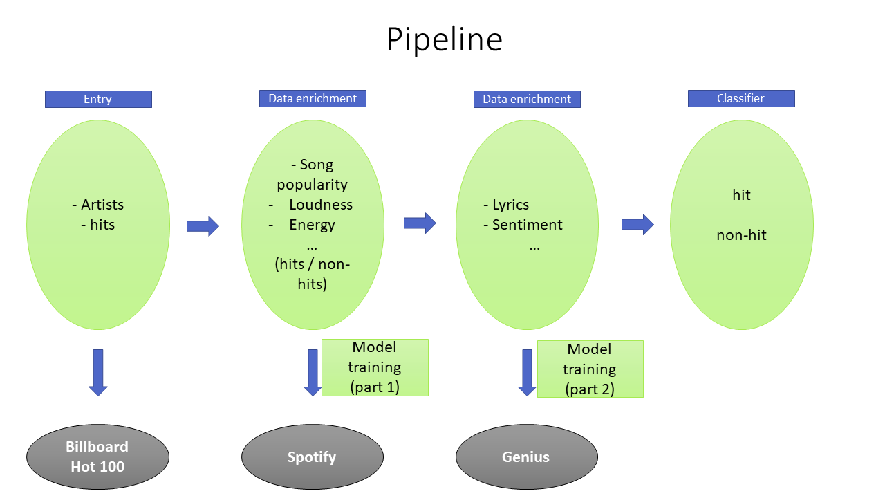
My data

我的資料

I couldn’t have a data set from a single source that contained all the variables. To overcome this problem, I have resorted to data enrichment techniques with the following three data sources: Billboard, Spotify and Genius.

我無法從包含所有變量的單一來源獲得數據集。 為了克服這個問題，我采用了以下三種數據源的數據豐富技術：Billboard，Spotify和Genius。

First, using Beautiful Soup, I collected a list of Billboard Year-End Hot 100 songs from 2010 to 2019, at the rate of 100 songs per year. Then, the Spotipy package was used for the recovery of data related to the songs audio characteristics such as danceability, instrumentalness, liveness, etc., on one hand; and, on the other hand, those related to the artist’s profile such as number of followers, popularity, etc. for both previously recovered hit and other non-hit songs from the same period.

首先，我使用Beautiful Soup收集了2010年至2019年的Billboard年終熱門100首歌曲列表，并且以每年100首歌曲的速度進行收集。 然后，一方面使用Spotipy包恢復與歌曲的音頻特性有關的數據，例如舞蹈性，器樂性，活潑性等； 另一方面，與藝術家個人資料相關的那些信息，例如先前恢復的熱門歌曲和同一時期的其他非熱門歌曲的關注者數量，受歡迎程度等。

And finally, Genius will be used mainly for retrieving the lyrics for all the songs that have been collected.

最后， Genius將主要用于檢索已收集的所有歌曲的歌詞。

A song in our data set is considered a hit if it made it to the Billboard Year-End Hot 100 chart at least once during any of the years in the reporting period. In other words, our model was tasked with predicting whether a song would make it to Billboard’s 100 most popular song list or not.

如果在報告期內的任何一年中，我們的數據集中的某首歌曲至少進入Billboard Year-End Hot 100排行榜一次，則該歌曲被視為熱門歌曲。 換句話說，我們的模型的任務是預測歌曲是否會進入Billboard的100首最受歡迎歌曲列表。

Tools used :

使用的工具 ：

• The spotipy package to access data from the Spotify music platform

  Spotipy包，用于從Spotify音樂平臺訪問數據

• seaborn and matplotlib for data visualization
  seaborn和matplotlib用于數據可視化
• pandas and numpy for data analysis
  熊貓和numpy進行數據分析
• LightGBM and the scikit-learn library for building and evaluating the model
  LightGBM和用于構建和評估模型的scikit-learn庫

Features

特征

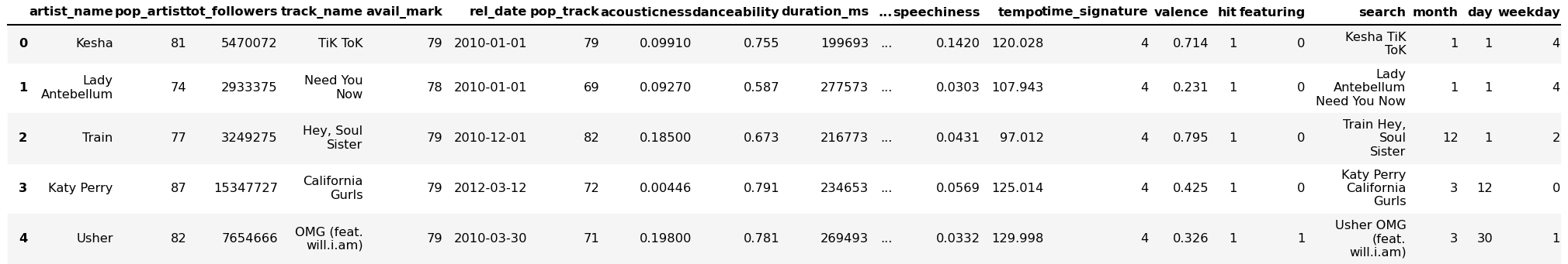
Spotify is one of the biggest streaming platforms in the world. Like Twitter or Facebook, it provides an API (Application Programming Interface) so that developers can interact with its huge music database. Via endpoints of this API, I was able to collect data for more than 22,000 songs; each song is characterized by more than twenty variables.

Spotify是世界上最大的流媒體平臺之一。 像Twitter或Facebook一樣，它提供了API(應用程序編程接口)，以便開發人員可以與其龐大的音樂數據庫進行交互。 通過該API的端點，我能夠收集超過22,000首歌曲的數據； 每首歌都有二十多個變量。

The variables returned by the API are as rich in information as they are varied. However, I have selected only those that are deemed relevant for the job. Then, they were transformed using feature engineering techniques in order to prepare the data set as well as possible for training the model. You will find the description of each of the variables used here. In general, the complete codes of the project are accessible through this link.

API返回的變量隨其變化而具有豐富的信息。 但是，我只選擇了與工作相關的那些。 然后，使用特征工程技術對它們進行轉換，以準備數據集并盡可能地訓練模型。 您將在此處找到每個變量的描述。 通常，可通過此鏈接訪問項目的完整代碼。

Some of these variables are used only for analysis, others are involved in all stages of the pipeline. Now let’s take a look at what the first five observations of our data set look like.

這些變量中的一些僅用于分析，而其他變量則涉及管道的所有階段。 現在，讓我們看一下數據集的前五個觀察結果。

Data visualization

數據可視化

Right before building the model, I wanted to explore the data a bit through visualizations; although the primary goal of the work was not to conduct a full exploratory analysis.

在建立模型之前，我想通過可視化來探索數據。 盡管這項工作的主要目標不是進行全面的探索性分析。

In light of the above graph, January is the month in which more hits were released; and July being the least requested one. We also notice that the majority of the hits for the period came out on the 4th day of the week; which is Thursday. Finally, the first day of the month is much more used to publish a song.

根據上面的圖表，一月份是發布更多匹配的月份； 而7月是要求最少的時間。 我們還注意到，該期間的大多數匹配均在一周的第4天發布； 這是星期四。 最后，每月的第一天更多地用于發布歌曲。

Based on that observation, we could deduce that publishing a song on January 1st is probably a step towards optimizing the chances of its virality. We must still be careful: correlation is not causation. We would have to push our analysis further in order to be more precise in this conclusion.

根據這一觀察，我們可以推斷出在1月1日發布歌曲可能是朝著優化病毒傳播機會邁出的一步。 我們仍然必須小心：關聯不是因果關系。 為了使該結論更加精確，我們將不得不進一步分析。

I continued the visualization, wanting to get an idea of ??which artists recorded the most hits over the period. Unsurprisingly, the graph below shows that artists like Drake, Rihanna, and Taylor Swift recorded more hits than anyone else during the period. That being said, it’s plausible to believe that a song is more likely to go viral if it contains the vocals of one of these artists.

我繼續進行可視化，想了解一下在這段時間內哪些藝術家記錄了最多的熱門歌曲。 毫不奇怪，下圖顯示了在這段時期內，德雷克(Drake)，蕾哈娜(Rihanna)和泰勒·斯威夫特(Taylor Swift)等藝術家錄得的熱門歌曲比其他任何人都多。 話雖這么說，相信一首歌如果包含其中一位藝術家的聲音，就更有可能傳播開來。

To understand what makes a song a hit; and another one not, it is imperative to study the audio-related variables of both categories. This is how I wanted to get an idea of ??the distribution of these variables with respect to the two categories.

了解什么使一首歌大受歡迎； 另一個不是，必須研究這兩種類別的音頻相關變量。 這就是我想要了解這些變量相對于兩個類別的分布的想法。

The predominant variables within the two categories are the same: energy, danceability and valence. The only difference is that the average values ??of these variables are higher for the hit songs category. This attests that the hits music are faster and more sonorous. They are more suited to dance and are more inclined to inspire joy, gaiety, euphoria.

這兩個類別中的主要變量相同：能量，舞蹈性和化合價。 唯一的區別是熱門歌曲類別的這些變量的平均值更高。 這證明了流行音樂的速度更快，聲音更大。 他們更適合跳舞，更容易激發歡樂，快樂和欣快感。

The machine learning approach

機器學習方法

So far we’ve been able to uncover some interesting insights about the data. In order to shorten this article, let’s go directly to the part about the machine learning algorithm that was used.

到目前為止 ，我們已經能夠發現有關數據的一些有趣的見解。 為了縮短本文的篇幅，讓我們直接轉到有關所使用的機器學習算法的部分。

I wanted to build a model to predict which class, hit or non-hit, that a song is most likely to belong to based on a set of explanatory variables, as explained at the beginning of this article.

我想建立一個模型，根據一組解釋性變量來預測一首歌曲最有可能屬于哪個類別(熱門還是非熱門)，如本文開頭所述。

In its raw state, the data collected was not ready for training a machine learning model. So I treated them; first, using the SMOTE technique, because the hit song class was under-represented compared to the non-hit category, then by using other feature engineering techniques in order to standardize the data.

在原始狀態下，收集的數據尚未準備好用于訓練機器學習模型。 所以我對待他們； 首先，使用SMOTE技術，因為與非熱門類別相比，熱門歌曲類別的代表性不足，然后使用其他特征工程技術來標準化數據。

Also, I wanted a model that would perform as well as possible. To do this, I trained several algorithms and compared the results based on the selected evaluation criteria. It turned out that the LightGBM classification algorithm is the one that, at the time of training, better detected the patterns between the explanatory variables and the variable to be predicted (hit).

另外，我想要一個性能最好的模型。 為此，我訓練了幾種算法，并根據選定的評估標準比較了結果。 事實證明，LightGBM分類算法是一種在訓練時可以更好地檢測解釋變量和要預測的變量(命中)之間的模式的算法。

%matplotlib inline
import lightgbm as lgb
from sklearn.metrics import auc, accuracy_score, roc_auc_score, roc_curve, confusion_matrix
from imblearn.over_sampling import SMOTE
from sklearn.model_selection import train_test_split
sm = SMOTE(random_state=42)X=df[['acousticness', 'danceability', 'energy', 'instrumentalness', 'liveness','loudness','speechiness', 'valence','tempo','duration_ms','featuring','pop_artist','tot_followers','avail_mark','pop_track']]
y=df['hit']# Spliting the data set
X_train, X_test, y_train, y_test = train_test_split(X, y, test_size=0.30, random_state=20)# Oversample the training data
X_res, y_res = sm.fit_resample(X_train, y_train)# Parameters optimized via GridSearch
clf = lgb.LGBMClassifier( boosting_type='gbdt', class_weight=None, colsample_bytree=1.0,importance_type='split', learning_rate=0.2, max_depth=-1,min_child_samples=20, min_child_weight=0.001, min_split_gain=0.0,n_estimators=90, n_jobs=-1, num_leaves=31, objective=None,random_state=None, reg_alpha=0.0, reg_lambda=0.0, silent=True,subsample=1.0, subsample_for_bin=200000, subsample_freq=0)clf.fit(X_res, y_res)

Confusion matrix

混淆矩陣

For a first level performance analysis of the model, we will use the confusion matrix. The visualization of the confusion matrix will allow us to understand the errors made by our classifier compared to the test subset.

對于模型的第一級性能分析，我們將使用混淆矩陣。 混淆矩陣的可視化將使我們能夠了解分類器與測試子集相比所犯的錯誤。

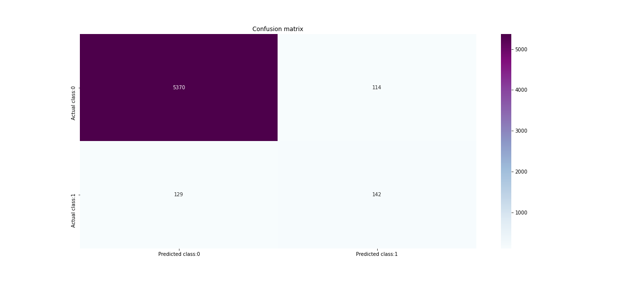
This matrix measures the quality of a classification system. In a binary classification, the principal diagonal represents the observations correctly classified by the model; and the secondary diagonal, those classified incorrectly. Therefore, the most frequent mistake made by the model is to have classified a song as non-hit when in reality it was a hit (129 cases), the type II error more precisely.

該矩陣衡量分類系統的質量。 在二元分類中，主對角線代表模型正確分類的觀測值； 以及次級對角線，則歸類不正確。 因此，該模型最常犯的錯誤是將一首歌曲實際上沒有擊中時將其歸類為未擊中(129例)，更準確地說是II型錯誤。

Type I error is that the model classifies song as a hit when it is non-hit (false hit); and type II error, the reverse; that is to say the case where it classifies a music as non-hit yet it is hit (false non-hit). If we are trying to understand the psychology of a music producer, Type I error is less acceptable than Type II error. We wouldn’t want to incur all the expenses related to the production and promotion of a song that a model has predicted that would be a hit so that in the end it won’t be. The value of the Type I error should be minimal.

類型I錯誤是模型在歌曲未擊中(錯誤擊中)時將歌曲歸類為擊中； 和II型錯誤，反之； 也就是說，將音樂歸類為非流行但仍被流行(假非流行)的情況。 如果我們試圖了解音樂制作人的心理，則類型I錯誤比類型II錯誤更不可接受。 我們不想承擔模型制作所預想會很成功的歌曲制作和推廣相關的所有費用，因此最終不會出現。 類型I錯誤的值應該最小。

The classification report

分類報告

The classification report presents statistics calculated from the data in the confusion matrix. Each metric describes a different aspect of the classification. We will use this report for a second level performance analysis of the model.

分類報告提供了根據混淆矩陣中的數據計算出的統計信息。 每個度量標準都描述了分類的不同方面。 我們將使用此報告對該模型進行第二級性能分析。

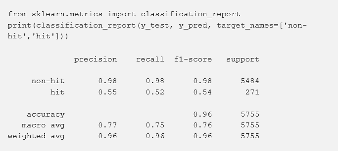
The accuracy, which globally measures the percentage of correct classification performed by the model, is 96%. Since the test subset is unbalanced, this percentage is stretched by the over-represented class, in this case, the non-hit class. So this metric is not the best we could use.

準確性(整體衡量模型執行的正確分類的百分比)為96％。 由于測試子集是不平衡的，因此該百分比會被過度代表的類(在這種情況下為非命中類)所擴展。 因此，該指標不是我們可以使用的最佳指標。

The recall measures the percentage of occurrences classified correctly by the model for each class. A classification is correct when the predicted class matches the actual class. On one hand, from the 5,484 non-hit songs that we used to test the model, 98% were correctly classified. On the other hand, the algorithm correctly classified only 52% of the 271 hit songs we submitted to it. You will have understood: it is more difficult for the algorithm to classify a hit song as a hit (true hit) than to classify a non-hit song as a non-hit (true non-hit).

召回度量模型為每個類別正確分類的出現百分比。 當預測的類別與實際類別匹配時，分類是正確的。 一方面，從我們用來測試模型的5,484首非熱門歌曲中，有98％被正確分類。 另一方面，該算法僅正確分類了我們提交給它的271首熱門歌曲中的52％。 您將了解：與將非流行歌曲分類為非流行歌曲(真正非流行)相比，算法將流行歌曲分類為流行歌曲(真正流行)要困難得多。

The precision levels for the non-hit and hit classes are 0.98 and 0.55, respectively. This translates that 98% of all the songs the model classified as non-hits are indeed non-hits; and, only 55% of the songs it predicted hits really are.

非命中和命中類別的精度水平分別為0.98和0.55。 這意味著該模型分類為非流行歌曲的所有歌曲中有98％確實是非流行歌曲。 而且，它預測的熱門歌曲中只有55％確實是。

Our model reacts better when it comes to non-hits songs. This is most likely due to the fact that from the start this class had a lot more data. The pattern detection between the non-hit modality of the dependent variable and the other explanatory variables is perhaps favored because of this.

對于非熱門歌曲，我們的模型React更好。 這很可能是由于該類從一開始就擁有很多數據這一事實。 因此，可能更喜歡在因變量的非命中模態和其他解釋變量之間進行模式檢測。

Once satisfied with the performance of the model, I resolved to understand the most influential explanatory variables in determining the class of a given song. That’s why I used the plot importance below.

對模型的性能感到滿意后，我決定了解最有影響力的解釋變量，以確定給定歌曲的類別。 這就是為什么我在下面使用情節重要性。

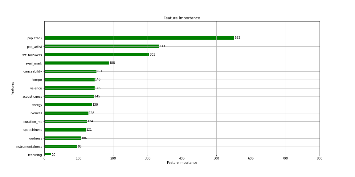
We can see that the popularity of a song on Spotify is the most important variable in the process of predicting which class it is most likely to belong to. Then, the artist’s popularity on Spotify, the number of followers he has and the number of markets in which the song is available on constitutes a second wave of determining variables in the process. Finally come mainly the variables related to the audio of the songs with a relatively similar level of influence.

我們可以看到，在預測歌曲最有可能屬于哪個類別的過程中，Spotify上歌曲的流行程度是最重要的變量。 然后，藝術家在Spotify上的受歡迎程度，他所擁有的追隨者數量以及歌曲可在其上獲得的市場數量構成了第二個確定變量的過程。 最后主要是影??響力相對相似的與歌曲音頻相關的變量。

This analysis draws attention to something major. Essentially, a song is a hit if it is popular on Spotify, is performed by an artist who is also popular on Spotify and has a significant number of followers, and finally, if it is available in the greatest number of countries across the world. This conclusion seems logical, and … Eurêka🙂, it is also verified empirically by our model.

該分析將注意力吸引到主要方面。 從本質上講，如果歌曲在Spotify上很流行，那么它就是一首熱門歌曲，這是由一位在Spotify上也很受歡迎并且有大量追隨者的藝術家表演的，最后，如果它在世界上最多的國家/地區都有銷售。 這個結論似乎是合乎邏輯的，而且…Eurêka🙂，我們的模型也通過經驗進行了驗證。

To better appreciate the relevance of this conclusion, it should be borne in mind that Billboard’s year-end top 100 music list is based primarily on a commercial aspect. Indeed, this ranking is a faithful reflection of physical and digital sales, radio listening and music streaming in the United States; all income-generating activities, directly or indirectly.

為了更好地理解此結論的相關性，應該牢記Billboard的年終前100名音樂榜單主要基于商業方面。 實際上，該排名真實反映了美國的實體和數字銷售，廣播收聽和音樂流； 所有直接或間接產生收入的活動。

The more popular the song is on Spotify, the more it is listened to online.; more streams translates to more revenue generated because after each song listened to by a subscriber, the streaming platforms pay a fee to the artist or the music label. The popularity of the artist on Spotify and the number of followers he has there are channels that amplify the number of streams and sales, which will then help increase the income generated by his music.

這首歌在Spotify上越流行，在線上收聽的次數就越多。 更多的流轉化為更多的收入，因為在訂閱者聽完每首歌曲之后，流平臺向藝術家或音樂唱片公司收取費用。 藝術家在Spotify上的受歡迎程度以及他擁有的追隨者數量，這些渠道可以擴大流媒體的數量和銷量，從而有助于增加他的音樂產生的收入。

The more revenue music generates, the more likely it is to be on Billboard’s top 100 music list at the end of the year; therefore the more likely it is also to be ranked hit by our model because the variables that mainly determine the level of music income are the most influential in the ranking process according to our importance graph (logical, isn’t it😉 ?).

音樂產生的收入越多，到年底它就更有可能進入Billboard的前100名音樂榜單； 因此，根據我們的重要性圖，主要決定音樂收入水平的變量在排名過程中最具影響力，因此我們的模型也更有可能對其進行排名排名(邏輯上不是嗎？)。

Usually, songs have another important characteristic that we haven’t yet taken into account: the lyrics. Can we further increase the performance of the model by using lyrics? This is what we will explore in the second part of the article.

通常，歌曲具有我們尚未考慮的另一個重要特征：歌詞。 我們可以通過使用歌詞進一步提高模型的性能嗎？ 這就是我們將在本文的第二部分中探討的內容。

As always I welcome constructive criticism and feedback. I can be reached on Twitter @jbobym.

一如既往，我歡迎建設性的批評和反饋。 可以通過Twitter @ jbobym與我聯系 。