Canny邊緣檢測算法背景
求邊緣幅度的算法:
一階導數:sobel、Roberts、prewitt等算子
二階導數:Laplacian、Canny算子
Canny算子效果比其他的都要好,但是實現起來有點麻煩
Canny邊緣檢測算法的優勢:
Canny是目前最優秀的邊緣檢測算法,其目標為找到一個最優的邊緣,其最優邊緣的定義為:
1、好的檢測:算法能夠盡可能的標出圖像中的實際邊緣
2、好的定位:標識出的邊緣要與實際圖像中的邊緣盡可能接近
3、最小響應:圖像中的邊緣只能標記一次
Canny邊緣檢測算法的實現方法:
1.對圖像進行灰度化:
方法1:Gray=(R+G+B)/3;
方法2:Gray=0.299R+0.587G+0.114B;(這種參數考慮到了人眼的生理特點)
2.對圖像進行高斯濾波: 根據待濾波的像素點及其鄰域點的灰度值按照一定的參數規則進行加權平均。這樣 可以有效濾去理想圖像中疊加的高頻噪聲。
3. 檢測圖像中的水平、垂直和對角邊緣(如Prewitt,Sobel算子等)。
4. 對梯度幅值進行非極大值抑制
5. 用雙閾值算法檢測和連接邊緣
高斯平滑
高斯平滑水平和垂直方向呈現高斯分布,更突出了 中心點在像素平滑后的權重,相比于均值濾波而言, 有著更好的平滑效果。
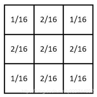
高斯平滑水平和垂直方向呈現高斯分布,更突出了中心點在像素平滑后的權重,相比于均值濾波 而言,有著更好的平滑效果。
重要的是需要理解,高斯卷積核大小的選擇將影響Canny檢測器的性能: 尺寸越大,檢測器對噪聲的敏感度越低,但是邊緣檢測的定位誤差也將略有增加。一般5x5是一個 比較不錯的trade off。
非極大值抑制
非極大值抑制,簡稱為NMS算法,英文為Non-Maximum Suppression。 其思想是搜素局部最大值,抑制極大值。 NMS算法在不同應用中的具體實現不太一樣,但思想是一樣的。
為什么要用非極大值抑制?
以目標檢測為例:目標檢測的過程中在同一目標的位置上會產生大量的候選框,這些候選框相互之間可 能會有重疊,此時我們需要利用非極大值抑制找到最佳的目標邊界框,消除冗余的邊界框。
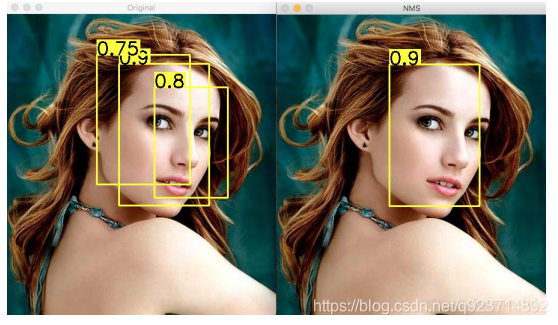
對于重疊的候選框,若大于規定閾值(某一提前設定的置信度),則刪除;低于閾值則保留。 對于無重疊的候選框,都保留。
實現方法:
1.將當前像素的梯度強度與沿正負梯度方向上的兩個像素進行比較。
2.如果當前像素的梯度強度與另外兩個像素相比最大,則該像素點保留為邊緣點,否則 該像素點將被抑制(灰度值置為0)。
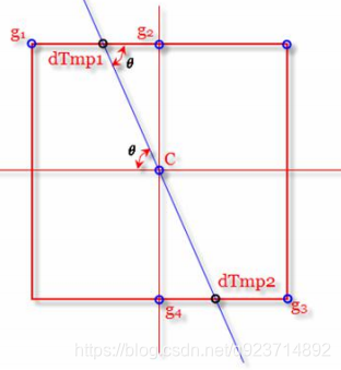
例如這個圖,點C是我們最大值,但是我們要知道是不是局部最大值,就看我們事先求出的該點梯度線,梯度線周圍臨近像素點取交叉點dTmp1與dTmp2,若dTmp1與dTmp2的灰度值都比c點大,該點將被舍棄,只有該點的灰度值大于dTmp1與dTmp2的灰度值才能被保留。
用雙閾值算法檢測(滯后閾值)
完成非極大值抑制后,會得到一個二值圖像,非邊緣的點灰度值均為0,可能為邊緣的局部灰度極大值點可設置其灰度為128。 這樣一個檢測結果還是包含了很多由噪聲及其他原因造成的假邊緣。因此還需要進一步的 處理。 用雙閾值算法檢測(滯后閾值)
? 如果邊緣像素的梯度值高于高閾值,則將其標記為強邊緣像素;
? 如果邊緣像素的梯度值小于高閾值并且大于低閾值,則將其標記為弱邊緣像素;
? 如果邊緣像素的梯度值小于低閾值,則會被抑制。
雙閾值檢測: 大于高閾值為強邊緣,小于低閾值不是邊緣。介于中間是弱邊緣。 閾值的選擇取決于給定輸入圖像的內容。
抑制孤立低閾值點
到目前為止,被劃分為強邊緣的像素點已經被確定為邊緣,因為它們是從圖像中的真實邊緣中提取 出來的。 然而,對于弱邊緣像素,將會有一些爭論,因為這些像素可以從真實邊緣提取也可以是因噪聲或顏 色變化引起的。 為了獲得準確的結果,應該抑制由后者引起的弱邊緣:
? 通常,由真實邊緣引起的弱邊緣像素將連接到強邊緣像素,而噪聲響應未連接。
? 為了跟蹤邊緣連接,通過查看弱邊緣像素及其8個鄰域像素,只要其中一個為強邊緣像素, 則該弱邊緣點就可以保留為真實的邊緣。
Canny邊緣檢測算法的代碼手動實現:
import numpy as np
import matplotlib.pyplot as plt
import mathif __name__ == '__main__':pic_path = 'lenna.png' img = plt.imread(pic_path)if pic_path[-4:] == '.png':  # .png圖片在這里的存儲格式是0到1的浮點數,所以要擴展到255再計算img = img * 255  # 還是浮點數類型img = img.mean(axis=-1)  # 取均值就是灰度化了# 1、高斯平滑#sigma = 1.52  # 高斯平滑時的高斯核參數,標準差,可調sigma = 0.5  # 高斯平滑時的高斯核參數,標準差,可調dim = int(np.round(6 * sigma + 1))  # round是四舍五入函數,根據標準差求高斯核是幾乘幾的,也就是維度if dim % 2 == 0:  # 最好是奇數,不是的話加一dim += 1Gaussian_filter = np.zeros([dim, dim])  # 存儲高斯核,這是數組不是列表了tmp = [i-dim//2 for i in range(dim)]  # 生成一個序列n1 = 1/(2*math.pi*sigma**2)  # 計算高斯核n2 = -1/(2*sigma**2)for i in range(dim):for j in range(dim):Gaussian_filter[i, j] = n1*math.exp(n2*(tmp[i]**2+tmp[j]**2))Gaussian_filter = Gaussian_filter / Gaussian_filter.sum()dx, dy = img.shapeimg_new = np.zeros(img.shape)  # 存儲平滑之后的圖像,zeros函數得到的是浮點型數據tmp = dim//2img_pad = np.pad(img, ((tmp, tmp), (tmp, tmp)), 'constant')  # 邊緣填補for i in range(dx):for j in range(dy):img_new[i, j] = np.sum(img_pad[i:i+dim, j:j+dim]*Gaussian_filter)plt.figure(1)plt.imshow(img_new.astype(np.uint8), cmap='gray')  # 此時的img_new是255的浮點型數據,強制類型轉換才可以,gray灰階plt.axis('off')# 2、求梯度。以下兩個是濾波求梯度用的sobel矩陣(檢測圖像中的水平、垂直和對角邊緣)sobel_kernel_x = np.array([[-1, 0, 1], [-2, 0, 2], [-1, 0, 1]])sobel_kernel_y = np.array([[1, 2, 1], [0, 0, 0], [-1, -2, -1]])img_tidu_x = np.zeros(img_new.shape)  # 存儲梯度圖像img_tidu_y = np.zeros([dx, dy])img_tidu = np.zeros(img_new.shape)img_pad = np.pad(img_new, ((1, 1), (1, 1)), 'constant')  # 邊緣填補,根據上面矩陣結構所以寫1for i in range(dx):for j in range(dy):img_tidu_x[i, j] = np.sum(img_pad[i:i+3, j:j+3]*sobel_kernel_x)  # x方向img_tidu_y[i, j] = np.sum(img_pad[i:i+3, j:j+3]*sobel_kernel_y)  # y方向img_tidu[i, j] = np.sqrt(img_tidu_x[i, j]**2 + img_tidu_y[i, j]**2)img_tidu_x[img_tidu_x == 0] = 0.00000001angle = img_tidu_y/img_tidu_xplt.figure(2)plt.imshow(img_tidu.astype(np.uint8), cmap='gray')plt.axis('off')# 3、非極大值抑制img_yizhi = np.zeros(img_tidu.shape)for i in range(1, dx-1):for j in range(1, dy-1):flag = True  # 在8鄰域內是否要抹去做個標記temp = img_tidu[i-1:i+2, j-1:j+2]  # 梯度幅值的8鄰域矩陣if angle[i, j] <= -1:  # 使用線性插值法判斷抑制與否num_1 = (temp[0, 1] - temp[0, 0]) / angle[i, j] + temp[0, 1]num_2 = (temp[2, 1] - temp[2, 2]) / angle[i, j] + temp[2, 1]if not (img_tidu[i, j] > num_1 and img_tidu[i, j] > num_2):flag = Falseelif angle[i, j] >= 1:num_1 = (temp[0, 2] - temp[0, 1]) / angle[i, j] + temp[0, 1]num_2 = (temp[2, 0] - temp[2, 1]) / angle[i, j] + temp[2, 1]if not (img_tidu[i, j] > num_1 and img_tidu[i, j] > num_2):flag = Falseelif angle[i, j] > 0:num_1 = (temp[0, 2] - temp[1, 2]) * angle[i, j] + temp[1, 2]num_2 = (temp[2, 0] - temp[1, 0]) * angle[i, j] + temp[1, 0]if not (img_tidu[i, j] > num_1 and img_tidu[i, j] > num_2):flag = Falseelif angle[i, j] < 0:num_1 = (temp[1, 0] - temp[0, 0]) * angle[i, j] + temp[1, 0]num_2 = (temp[1, 2] - temp[2, 2]) * angle[i, j] + temp[1, 2]if not (img_tidu[i, j] > num_1 and img_tidu[i, j] > num_2):flag = Falseif flag:img_yizhi[i, j] = img_tidu[i, j]plt.figure(3)plt.imshow(img_yizhi.astype(np.uint8), cmap='gray')plt.axis('off')# 4、雙閾值檢測,連接邊緣。遍歷所有一定是邊的點,查看8鄰域是否存在有可能是邊的點,進棧lower_boundary = img_tidu.mean() * 0.5high_boundary = lower_boundary * 3  # 這里我設置高閾值是低閾值的三倍zhan = []for i in range(1, img_yizhi.shape[0]-1):  # 外圈不考慮了for j in range(1, img_yizhi.shape[1]-1):if img_yizhi[i, j] >= high_boundary:  # 取,一定是邊的點img_yizhi[i, j] = 255zhan.append([i, j])elif img_yizhi[i, j] <= lower_boundary:  # 舍img_yizhi[i, j] = 0while not len(zhan) == 0:temp_1, temp_2 = zhan.pop()  # 出棧a = img_yizhi[temp_1-1:temp_1+2, temp_2-1:temp_2+2]if (a[0, 0] < high_boundary) and (a[0, 0] > lower_boundary):img_yizhi[temp_1-1, temp_2-1] = 255  # 這個像素點標記為邊緣zhan.append([temp_1-1, temp_2-1])  # 進棧if (a[0, 1] < high_boundary) and (a[0, 1] > lower_boundary):img_yizhi[temp_1 - 1, temp_2] = 255zhan.append([temp_1 - 1, temp_2])if (a[0, 2] < high_boundary) and (a[0, 2] > lower_boundary):img_yizhi[temp_1 - 1, temp_2 + 1] = 255zhan.append([temp_1 - 1, temp_2 + 1])if (a[1, 0] < high_boundary) and (a[1, 0] > lower_boundary):img_yizhi[temp_1, temp_2 - 1] = 255zhan.append([temp_1, temp_2 - 1])if (a[1, 2] < high_boundary) and (a[1, 2] > lower_boundary):img_yizhi[temp_1, temp_2 + 1] = 255zhan.append([temp_1, temp_2 + 1])if (a[2, 0] < high_boundary) and (a[2, 0] > lower_boundary):img_yizhi[temp_1 + 1, temp_2 - 1] = 255zhan.append([temp_1 + 1, temp_2 - 1])if (a[2, 1] < high_boundary) and (a[2, 1] > lower_boundary):img_yizhi[temp_1 + 1, temp_2] = 255zhan.append([temp_1 + 1, temp_2])if (a[2, 2] < high_boundary) and (a[2, 2] > lower_boundary):img_yizhi[temp_1 + 1, temp_2 + 1] = 255zhan.append([temp_1 + 1, temp_2 + 1])for i in range(img_yizhi.shape[0]):for j in range(img_yizhi.shape[1]):if img_yizhi[i, j] != 0 and img_yizhi[i, j] != 255:img_yizhi[i, j] = 0# 繪圖plt.figure(4)plt.imshow(img_yizhi.astype(np.uint8), cmap='gray')plt.axis('off')  # 關閉坐標刻度值plt.show()
Canny邊緣檢測算法的代碼實現:
import cv2
import numpy as np'''
cv2.Canny(image, threshold1, threshold2[, edges[, apertureSize[, L2gradient ]]])
必要參數:
第一個參數是需要處理的原圖像,該圖像必須為單通道的灰度圖;
第二個參數是滯后閾值1;
第三個參數是滯后閾值2。
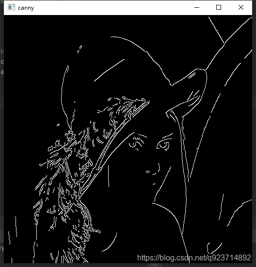
'''img = cv2.imread("lenna.png", 1)
gray = cv2.cvtColor(img, cv2.COLOR_BGR2GRAY)
cv2.imshow("canny", cv2.Canny(gray, 200, 300))
cv2.waitKey()
cv2.destroyAllWindows()輸出結果:
額外內容:
可動態調整Canny邊緣檢測閾值的算法
上圖的雙閾值我們設置的是[200,300]
實際上Canny邊緣檢測算法中閾值的影響非常大,為了方便理解,老師編寫了一個可動態調整閾值的算法。
import cv2
import numpy as np def CannyThreshold(lowThreshold):  detected_edges = cv2.GaussianBlur(gray,(3,3),0) #高斯濾波 detected_edges = cv2.Canny(detected_edges,lowThreshold,lowThreshold*ratio,apertureSize = kernel_size)  #邊緣檢測# just add some colours to edges from original image.  dst = cv2.bitwise_and(img,img,mask = detected_edges)  #用原始顏色添加到檢測的邊緣上cv2.imshow('canny demo',dst)  lowThreshold = 0
max_lowThreshold = 200
ratio = 3
kernel_size = 3  img = cv2.imread('lenna.png')
gray = cv2.cvtColor(img,cv2.COLOR_BGR2GRAY)  #轉換彩色圖像為灰度圖cv2.namedWindow('canny demo')  #設置調節杠,
'''
下面是第二個函數,cv2.createTrackbar()
共有5個參數,其實這五個參數看變量名就大概能知道是什么意思了
第一個參數,是這個trackbar對象的名字
第二個參數,是這個trackbar對象所在面板的名字
第三個參數,是這個trackbar的默認值,也是調節的對象
第四個參數,是這個trackbar上調節的范圍(0~count)
第五個參數,是調節trackbar時調用的回調函數名
'''
cv2.createTrackbar('Min threshold','canny demo',lowThreshold, max_lowThreshold, CannyThreshold)  CannyThreshold(0)  # initialization
if cv2.waitKey(0) == 27:  #wait for ESC key to exit cv2cv2.destroyAllWindows()
實驗結果:
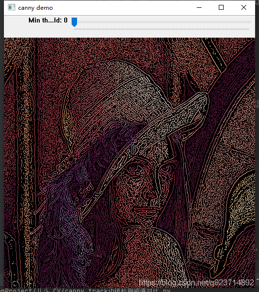
0閾值時:
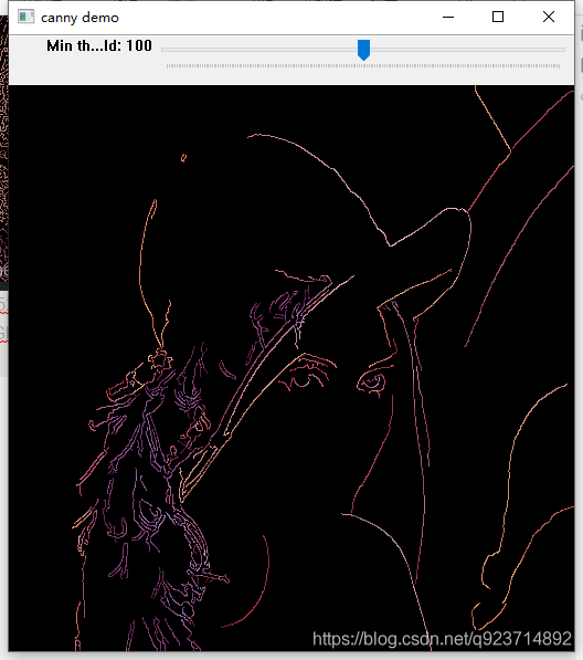
100閾值時:
200閾值時:
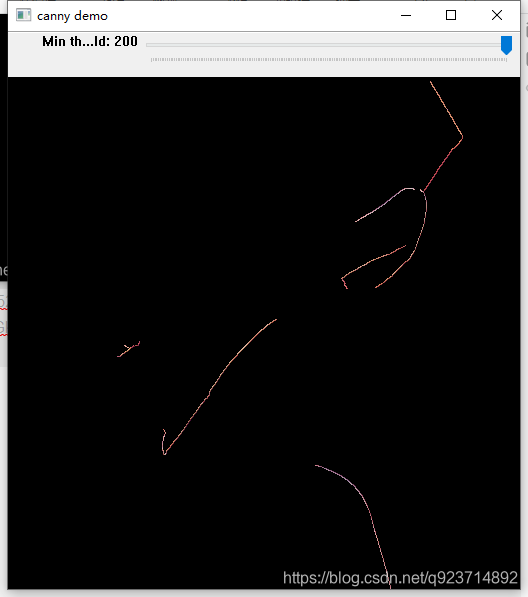
閾值越大,能夠保留了邊緣越少
Sobel,Laplace,Canny邊緣檢測的效果對比:
import cv2
import numpy as np
from matplotlib import pyplot as plt  img = cv2.imread("lenna.png",1)  img_gray = cv2.cvtColor(img, cv2.COLOR_RGB2GRAY)  '''
Sobel算子
Sobel算子函數原型如下:
dst = cv2.Sobel(src, ddepth, dx, dy[, dst[, ksize[, scale[, delta[, borderType]]]]])
前四個是必須的參數:
第一個參數是需要處理的圖像;
第二個參數是圖像的深度,-1表示采用的是與原圖像相同的深度。目標圖像的深度必須大于等于原圖像的深度;
dx和dy表示的是求導的階數,0表示這個方向上沒有求導,一般為0、1、2。
其后是可選的參數:
dst是目標圖像;
ksize是Sobel算子的大小,必須為1、3、5、7。
scale是縮放導數的比例常數,默認情況下沒有伸縮系數;
delta是一個可選的增量,將會加到最終的dst中,同樣,默認情況下沒有額外的值加到dst中;
borderType是判斷圖像邊界的模式。這個參數默認值為cv2.BORDER_DEFAULT。
'''img_sobel_x = cv2.Sobel(img_gray, cv2.CV_64F, 1, 0, ksize=3)  # 對x求導
img_sobel_y = cv2.Sobel(img_gray, cv2.CV_64F, 0, 1, ksize=3)  # 對y求導# Laplace 算子
img_laplace = cv2.Laplacian(img_gray, cv2.CV_64F, ksize=3)  # Canny 算子
img_canny = cv2.Canny(img_gray, 100 , 150)  plt.subplot(231), plt.imshow(img_gray, "gray"), plt.title("Original")
plt.subplot(232), plt.imshow(img_sobel_x, "gray"), plt.title("Sobel_x")
plt.subplot(233), plt.imshow(img_sobel_y, "gray"), plt.title("Sobel_y")
plt.subplot(234), plt.imshow(img_laplace,  "gray"), plt.title("Laplace")
plt.subplot(235), plt.imshow(img_canny, "gray"), plt.title("Canny")
plt.show()
實現結果:
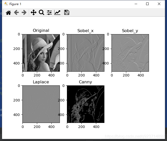
從實驗結果可以發現,在邊緣檢測的效果上,Canny > Laplace > Sobel


DDL增強功能-數據類型、同義詞、分區表)

初衷、感想與筆記目錄)


_主成分分析技巧)


