介紹 (Introduction)

Principal Component Analysis (PCA) is an unsupervised technique for dimensionality reduction.

主成分分析(PCA)是一種無監督的降維技術。

What is dimensionality reduction?

什么是降維？

Let us start with an example. In a tabular data set, each column would represent a feature, or dimension. It is commonly known that it is difficult to manipulate a tabular data set that has a lot of columns/features, especially if there are more columns than observations.

讓我們從一個例子開始。 在表格數據集中，每列將代表一個要素或尺寸。 眾所周知，很難處理具有許多列/功能的表格數據集，尤其是當列數多于觀察值時。

Given a linearly modelable problem having a number of features p=40, then the best subset approach would fit a about trillion (2^p-1) possible models and submodels, making their computation extremely onerous.

給定一個具有多個特征p = 40的線性可建模問題，那么最佳子集方法將適合大約一萬億(2 ^ p-1)個可能的模型和子模型，從而使其計算極為繁瑣。

How does PCA come to aid?

PCA如何提供幫助？

PCA can extract information from a high-dimensional space (i.e., a tabular data set with many columns) by projecting it onto a lower-dimensional subspace. The idea is that the projection space will have dimensions, named principal components, that will explain the majority of the variation of the original data set.

PCA可以通過將其投影到低維子空間上來 從高維空間 (即具有許多列的表格數據集)中提取信息 。 這個想法是，投影空間將具有稱為主成分的維，這些維將解釋原始數據集的大部分變化。

How does PCA work exactly?

PCA如何工作？

PCA is the eigenvalue decomposition of the covariance matrix obtained after centering the features, to find the directions of maximum variation. The eigenvalues represent the variance explained by each principal component.

PCA是對特征進行居中后找到最大變化方向的協方差矩陣的特征值分解。 特征值代表每個主成分所解釋的方差。

The purpose of PCA is to obtain an easier and faster way to both manipulate data set (reducing its dimensions) and retain most of the original information through the explained variance.

PCA的目的是獲得一種更簡便，更快捷的方式來處理數據集(減小其尺寸)并通過所解釋的差異保留大多數原始信息。

The question now is

現在的問題是

How many components should I use for dimensionality reduction? What is the “right” number?

我應該使用幾個零件來減少尺寸？ 什么是“正確的”數字？

In this post, we will discuss some tips for selecting the optimal number of principal components by providing practical examples in Python, by:

在本文中，我們將通過在Python中提供一些實用的示例，討論一些用于選擇最佳數量的主要組件的技巧，方法如下：

1. Observing the cumulative ratio of explained variance.
   觀察解釋方差的累積比率。
2. Observing the eigenvalues of the covariance matrix
   觀察協方差矩陣的特征值
3. Tuning the number of components as hyper-parameter in a cross-validation framework where PCA is applied in a Machine Learning pipeline.
   在交叉驗證框架中將組件的數量調整為超參數，在交叉驗證框架中將PCA應用到機器學習管道中。

Finally, we will also apply dimensionality reduction on a new observation, in the scenario where PCA was already applied to a data set, and we would like to project the new observation on the previously obtained subspace.

最后，在已經將PCA應用于數據集的情況下，我們還將對新觀測值進行降維 ，并且我們希望將新觀測值投影到先前獲得的子空間上。

環境設置 (Environment set-up)

At first, we import the modules we will be using, and load the “Breast Cancer Data Set”: it contains 569 observations and 30 features for relevant clinical information — such as radius, texture, perimeter, area, etc. — computed from digitized image of aspirates of breast masses, and it presents a binary classification problem, as the labes are only 0 or 1 (benign vs malignant), indicating whether a patient has breast cancer or not.

首先，我們導入將要使用的模塊，并加載“ 乳腺癌數據集 ”：它包含569個觀察值和30個相關臨床信息的特征(例如半徑，紋理，周長，面積等)，這些特征是通過數字化計算得出的乳腺抽吸物的圖像，它提出了一個二元分類問題 ，因為標記只有0或1(良性與惡性)，表明患者是否患有乳腺癌。

The data set is already available in scikit-learn:

數據集已在scikit-learn中提供：

Without diving deep into the pre-processing task, it is important to mention that the PCA is affected by different scales in the data.

在不深入研究預處理任務的情況下，重要的是要提到PCA受數據中不同比例的影響。

Therefore, before applying PCA the data must be scaled (i.e., converted to have mean=0 and variance=1). This can be easily achieved with the scikit-learn StandardScaler object:

因此，在應用PCA之前， 必須對數據進行縮放 (即轉換為均值= 0和方差= 1)。 這可以通過scikit-learn StandardScaler對象輕松實現：

This returns:

返回：

Mean:  -6.118909323768877e-16
Standard Deviation:  1.0

Once the features are scaled, applying the PCA is straightforward. In fact, scikit-learn handles almost everything by itself: the user only has to declare the number of components and then fit.

縮放功能后，即可輕松應用PCA。 實際上，scikit-learn本身幾乎可以處理所有事情：用戶只需要聲明組件的數量即可。

Notably, the scikit-learn user can either declare the number of components to be used, or the ratio of explained variance to be reached:

值得注意的是，scikit-learn用戶可以聲明要使用的組件數量 ， 或要達到的解釋方差比率 ：

• pca = PCA(n_components=5): performs PCA using 5 components.

  pca = PCA(n_components = 5) ：使用5個組件執行PCA。

• pca = PCA(n_components=.95): performs PCA using a number of components sufficient to consider 95% of variance.

  pca = PCA(n_components = .95) ：使用足以考慮95％方差的多個分量執行PCA。

Indeed, this is a way to select the number of components: asking scikit-learn to reach a certain amount of explained variance, such as 95%. But maybe we could have used a significantly lower amount of dimensions and reach a similar variance, for example 92%.

確實，這是一種選擇組件數量的方法：要求scikit-learn達到一定的解釋方差，例如95％。 但是也許我們可以使用低得多的尺寸并達到類似的方差，例如92％。

So, how do we select the number of components?

那么，我們如何選擇組件數量？

1.觀察解釋方差的比率 (1. Observing the ratio of explained variance)

PCA achieves dimensionality reduction by projecting the observations on a smaller subspace, but we also want to keep as much information as possible in terms of variance.

PCA通過將觀測值投影在較小的子空間上來實現降維，但我們也希望在方差方面保留盡可能多的信息。

So, one heuristic yet effective approach is to see how much variance is explained by adding the principal components one by one, and afterwards select the number of dimensions that meet our expectations.

因此，一種啟發式但有效的方法是通過將主要成分一一添加來查看解釋了多少差異，然后選擇滿足我們期望的維數。

It is very easy to follow this approach thanks to scikit-learn, that provides the explained_variance_ratio_ property to the (fitted) PCA object:

借助scikit-learn，可以很容易地采用這種方法，該方法為(已安裝的)PCA對象提供了explained_variance_ratio_屬性：

From the plot, we can see that the first 6 components are sufficient to retain the 89% of the original variance.

從圖中可以看出，前6個分量足以保留原始方差的89％。

This is a good result, if we think that we started with a data set of 30 features, and that we could limit further analysis to only 6 dimensions without loosing too much information.

如果我們認為我們從30個要素的數據集開始，并且可以將進一步的分析限制在6個維度而又不丟失太多信息，那將是一個很好的結果。

2.使用協方差矩陣 (2. Using the covariance matrix)

Covariance is a measure of the “spread” of a set of observations around their mean value. When we apply PCA, what happens behind the curtain is that we apply a rotation to the covariance matrix of our data, in order to achieve a diagonal covariance matrix. In this way, we obtain data whose dimensions are uncorrelated.

協方差是對一組觀測值在其平均值附近的“分布”的度量。 當我們應用PCA時，幕后發生的事情是我們將旋轉應用于數據的協方差矩陣，以獲得對角協方差矩陣 。 通過這種方式，我們可以獲得維度不相關的數據 。

The diagonal covariance matrix obtained after transformation is the eigenvalue matrix, where the eigenvalues correspond to the variance explained by each component.

變換后獲得的對角協方差矩陣是特征值矩陣，其中特征值對應于每個組件解釋的方差。

Therefore, another approach to the selection of the ideal number of components is to look for an “elbow” in the plot of the eigenvalues.

因此， 選擇理想數量的零件的另一種方法是在特征值圖中尋找“彎頭”。

Let us observe the first elements of the covariance matrix of the principal components. As said, we expect it to be diagonal:

讓我們觀察主成分協方差矩陣的第一個元素。 如前所述，我們希望它是對角線的：

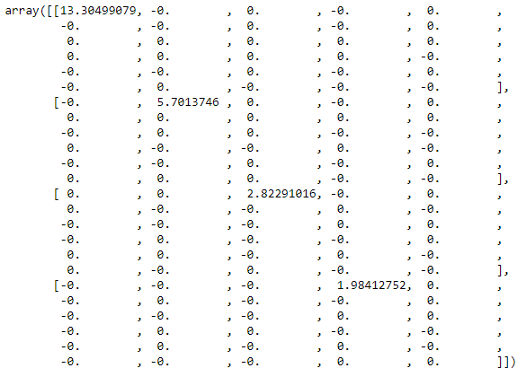
Indeed, at first glance the covariance matrix appears to be diagonal. In order to be sure that the matrix is diagonal, we can verify that all the values outside of the main diagonal are almost equal to zero (up to a certain decimal, as they will not be exactly zero).

確實，乍看之下，協方差矩陣似乎是對角線的。 為了確保矩陣是對角線，我們可以驗證主對角線之外的所有值幾乎都等于零(最多為某個小數，因為它們將不完全為零)。

We can use the assert_almost_equal statement, that leads to an exception in case its inner condition is not met, while it leads to no visible output in case the condition is met. In this case, no exception is raised (up to the tenth decimal):

我們可以使用assert_almost_equal語句，在不滿足其內部條件的情況下導致異常，而在滿足條件的情況下則導致不可見輸出。 在這種情況下，不會引發任何異常(最多十進制小數)：

The matrix is diagonal. Now we can proceed to plot the eigenvalues from the covariance matrix and look for an elbow in the plot.

矩陣是對角線的。 現在我們可以繼續繪制協方差矩陣的特征值，并在圖中尋找彎頭。

We use the diag method to extract the eigenvalues from the covariance matrix:

我們使用diag方法從協方差矩陣中提取特征值：

We may see an “elbow” around the sixth component, where the slope seems to change significantly.

我們可能會在第六部分周圍看到一個“彎頭”，那里的坡度似乎發生了很大變化。

Actually, all these steps were not needed: scikit-learn provides, among the others, the explained_variance_ attribute, defined in the documentation as “The amount of variance explained by each of the selected components. Equal to n_components largest eigenvalues of the covariance matrix of X.”:

實際上，不需要所有這些步驟：scikit-learn除其他外，還提供了explained_variance_屬性，該屬性在文檔中定義為“每個選定組件所解釋的方差量。 等于X的協方差矩陣的n_components個最大特征值。”：

In fact, we notice the same result as from the calculation of the covariance matrix and the eigenvalues.

實際上，我們注意到與計算協方差矩陣和特征值相同的結果。

3.應用交叉驗證程序 (3. Applying a cross-validation procedure)

Although PCA is an unsupervised technique, it might be used together with other techniques in a broader pipeline for a supervised problem.

盡管PCA是一種不受監督的技術，但它可以與其他技術一起在更廣泛的管道中用于受監督的問題。

For instance, we might have a classification (or regression) problem in a large data set, and we might apply PCA before our classification (or regression) model in order to reduce the dimensionality of the input dataset.

例如，我們可能在大型數據集中存在分類(或回歸)問題，并且我們可能在分類(或回歸)模型之前應用PCA，以降低輸入數據集的維數。

In this scenario, we would tune the number of principal components as a hyper-parameter within a cross-validation procedure.

在這種情況下，我們將在交叉驗證過程中將主成分的數量調整為超參數。

This can be achieved by using two scikit-learn object:

這可以通過使用兩個scikit-learn對象來實現：

• Pipeline: allows the definition of a pipeline of sequential steps in order to cross-validate them together.

  管道 ：允許定義順序步驟的管道，以便一起交叉驗證它們。

• GridSearchCV: performs a grid search in a cross-validation framework for hyper-parameter tuning (= finding the optimal parameters of the steps in the pipeline).

  GridSearchCV ：在交叉驗證框架中執行網格搜索以進行超參數調整 (=查找管線中步驟的最佳參數)。

The process is as follows:

流程如下：

1. The steps (dimensionality reduction, classification) are chained in a pipeline.
   步驟(降維，分類)鏈接在管道中。
2. The parameters to search are defined.
   已定義要搜索的參數。
3. The grid search procedure is executed.
   執行網格搜索過程。

In our example, we are facing a binary classification problem. Therefore, we apply PCA followed by logistic regression in a pipeline:

在我們的示例中，我們面臨一個二進制分類問題。 因此，我們在管道中應用PCA，然后進行邏輯回歸 ：

This returns:

返回：

Best parameters obtained from Grid Search:
{'log_reg__C': 1.2589254117941673, 'pca__n_components': 9}

The grid search finds the best number of components for the PCA during the cross-validation procedure.

網格搜索會在交叉驗證過程中找到PCA的最佳組件數量。

For our problem and tested parameters range, the best number of components is 9.

對于我們的問題和經過測試的參數范圍， 最佳組件數量是9 。

The grid search provides more detailed results in the cv_results_ attribute, that can be stored as a pandas dataframe and inspected:

網格搜索在cv_results_屬性中提供了更詳細的結果，可以將其存儲為pandas數據框并進行檢查：

As we can see, it contains detailed information on the cross-validated procedure with the grid search.

如我們所見，它包含有關通過網格搜索進行交叉驗證的過程的詳細信息。

But we might be not interested in seeing all the iterations performed by the grid search. Therefore, we can get the best validation score (averaged on all folds) for each number of components, and finally plot them together with the cumulative ratio of explained variance:

但是我們可能對查看網格搜索執行的所有迭代不感興趣。 因此，對于每種數量的組分，我們可以獲得最佳的驗證分數(在所有折疊中平均)，最后將它們與解釋的方差的累積比率一起繪制：

From the plot, we can notice that 6 components are enough to create a model whose validation accuracy reaches 97%, where considering all 30 components would lead to a 98% validation accuracy.

從圖中可以看出，只有6個組件足以創建一個驗證精度達到97％的模型，而考慮所有30個組件將得出98％的驗證精度 。

In a scenario with a significant number of features in a input data set, reducing the number of input features with PCA could lead to significant advantages in terms of:

在輸入數據集中有大量要素的情況下，使用PCA減少輸入要素的數量可能會帶來以下方面的顯著優勢：

1. Reduced training and prediction time.

   減少訓練和預測時間。

2. Increased scalability.

   增加可伸縮性。

3. Reduced training computational effort.

   減少訓練計算量。

While, at the same time, by choosing the optimal number of principal components in a pipeline for a supervised problem, tuning the hyper-parameter in a cross-validated procedure, we would ensure to retain optimal performances.

同時， 在同一時間 ，通過選擇一個監督問題的管線主要成分的最佳數量，調整超參數在交叉驗證過程中，我們會確保留住最佳的性能。

Although, it must be taken into account that in a data set with many features the PCA itself may prove computationally expensive.

但是，必須考慮到， 在具有許多功能的數據集中，PCA本身可能在計算上非常昂貴 。

如何將PCA應用于新觀測？ (How to apply PCA to a new observation?)

Now, let us suppose that we have applied the PCA to an existing data set and kept (for example) 6 components.

現在，讓我們假設已經將PCA應用于現有數據集并保留(例如)6個組件。

At some point, a new observation is added to the data set and needs to be projected on the reduced subspace obtained by PCA.

在某個時候， 新的觀測值會添加到數據集，并且需要投影到PCA獲得的縮小子空間上 。

How can this be achieved?

如何做到這一點？

We can perform this calculation manually through the projection matrix.

我們可以通過投影矩陣手動執行此計算。

Therefore, we also estimate the error in the manual calculation by checking if we would get the same output as “fit_transform” on the original data:

因此，我們還通過檢查是否在原始數據上獲得與“ fit_transform”相同的輸出來估計手動計算中的錯誤：

The projection matrix is orthogonal, and the manual reduction provides a fairly reasonable error.

投影矩陣是正交的，并且手動縮小提供了相當合理的誤差。

We can finally obtain the projection by the multiplication between the new observation (scaled) and the transposed projection matrix:

我們最終可以通過新觀測值(按比例縮放)與轉置投影矩陣之間的乘法來獲得投影：

This returns:

返回：

[-3.22877012 -1.17207348  0.26466433 -1.00294458  0.89446764  0.62922496]

That’s it! The new observation is projected to the 6-dimensional subspace obtained with PCA.

而已！ 新的觀測值投影到使用PCA獲得的6維子空間。

結論 (Conclusion)

This tutorial is meant to provide a few tips on the selection of the number of components to be used for the dimensionality reduction in the PCA, showing practical demonstrations in Python.

本教程旨在為您提供一些用于選擇PCA中降維的組件數量的技巧，并顯示Python的實際演示。

Finally, it is also explained how to perform the projection onto the reduced subspace of a new sample, information which is rarely found on tutorials on the subject.

最后，還說明了如何在新樣本的縮小子空間上進行投影，該信息在該主題的教程中很少見。

This is but a brief overview. The topic is far broader and it has been deeply investigated in literature.

這只是一個簡短的概述。 該主題范圍更廣，并且已在文獻中進行了深入研究。