一般線性模型和混合線性模型
生命科學的數學統計和機器學習 (Mathematical Statistics and Machine Learning for Life Sciences)
This is the eighteenth article from the column Mathematical Statistics and Machine Learning for Life Sciences where I try to explain some mysterious analytical techniques used in Bioinformatics and Computational Biology in a simple way. Linear Mixed Model (also called Linear Mixed Effects Model) is widely used in Life Sciences, there are many tutorials showing how to run the model in R, however it is sometimes unclear how exactly the Random Effects parameters are optimized in the likelihood maximization procedure. In my previous post How Linear Mixed Model Works I gave an introduction to the concepts of the model, and in this tutorial we will derive and code the Linear Mixed Model (LMM) from scratch applying the Maximum Likelihood (ML) approach, i.e. we will use plain R to code LMM and compare the output with the one from lmer and lme R functions. The goal of this tutorial is to explain LMM “like for my grandmother” implying that people with no mathematical background should be able to understand what LMM does under the hood.
這是生命科學的數學統計和機器學習專欄中的第18條文章,我試圖以一種簡單的方式來解釋一些在生物信息學和計算生物學中使用的神秘分析技術。 線性混合模型 (也稱為線性混合效應模型)在生命科學中被廣泛使用,有許多教程展示了如何在R中運行模型,但是有時不清楚在似然最大化過程中如何精確優化隨機效應參數。 在我以前的文章《線性混合模型的工作原理》中,我介紹了模型的概念,在本教程中,我們將使用最大似然(ML)方法從頭獲得并編碼線性混合模型(LMM),即我們將使用普通R編碼LMM并將輸出與lmer和lme R函數的輸出進行比較。 本教程的目的是“像祖母一樣”解釋LMM,這意味著沒有數學背景的人應該能夠理解LMM 在幕后的工作 。
玩具數據集 (Toy Data Set)
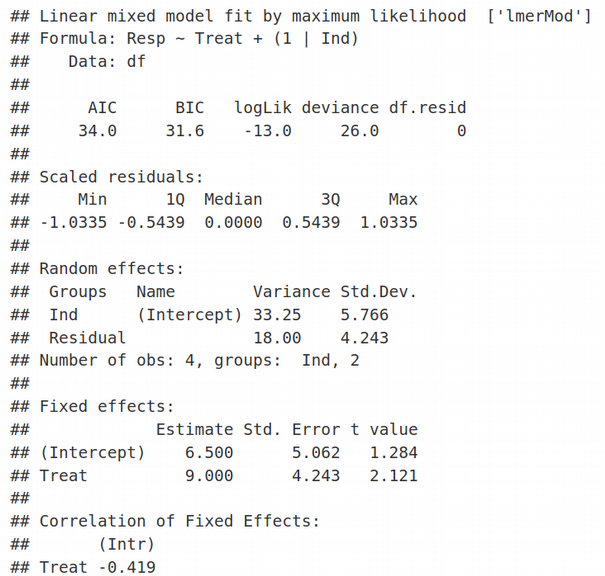
Let us consider a toy data set which is very simple but still keeps all necessary elements of the typical setup for Linear Mixed Modelling (LMM). Suppose we have only 4 data points / samples: 2 originating from Individual #1 and the other 2 coming from Individual #2. Further, the 4 points are spread between two conditions: untreated and treated. Let us assume we measure a response (Resp) of each individual to the treatment, and would like to address whether the treatment resulted in a significant response of the individuals in the study. In other words, we are aiming to implement something similar to the paired t-test and assess the significance of treatment. Later we will relate the outputs from LMM and paired t-test and show that they are indeed identical. In the toy data set, 0 in the Treat column implies “untreated”, and 1 means “treated”. First, we will use a naive Ordinary Least Squares (OLS) linear regression that does not take relatedness between the data points into account.
讓我們考慮一個非常簡單的玩具數據集 ,但它仍然保留了線性混合建模(LMM)典型設置的所有必要元素。 假設我們只有4個數據點 /樣本 :2 個數據源于#1個人 ,另外2 個數據源于#2個人 。 此外,這四個點分布在兩個條件之間: 未處理和已處理 。 讓我們假設我們測量了每個個體對治療的React( Resp ),并想說明治療是否導致研究中個體的顯著React。 換句話說,我們的目標是實施類似于 配對t檢驗的方法,并評估治療的重要性。 稍后,我們將把LMM和配對t檢驗的輸出相關聯,并證明它們確實是 相同的 。 在玩具的數據集,0在款待列意味著“未處理”,1分表示“經處理的”。 首先,我們將使用樸素的普通最小二乘(OLS) 線性回歸 ,該回歸不考慮數據點之間的相關性。
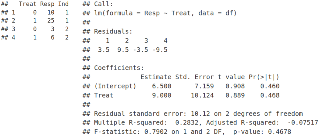
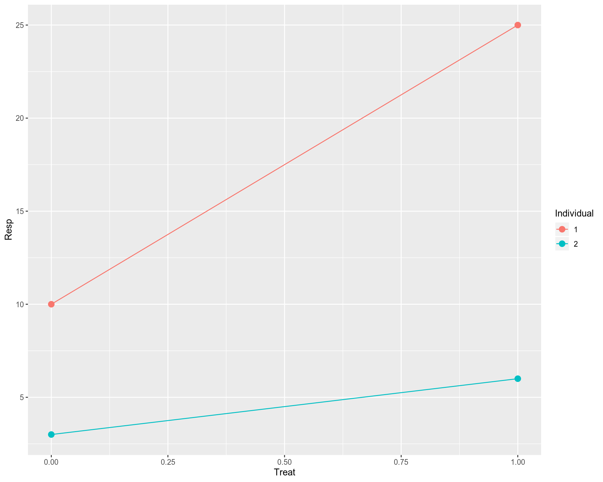
Technically it works, however, this is not a good fit, we have a problem here. Ordinary Least Squares (OLS) linear regression assumes that all observations (data points on the plot) are independent, that should result in uncorrelated and hence normally distributed residuals. However, we know that the data points on the plot belong to 2 individuals, i.e. 2 points for each individual. In principal, we can fit a linear model for each individual separately. However, this is not a good fit either. We have two points for each individual, so too few to make a reasonable fit for each individual. In addition, as we saw previously individual fits do not say much about the overall / population profile as some of them may have opposite behavior compared to the rest of individual fits.
從技術上講,它可以正常工作,但是,這不是一個很好的選擇, 我們 在這里 遇到了問題 。 普通最小二乘(OLS)線性回歸假設所有觀測值(圖中的數據點)都是獨立的 ,這將導致不相關且因此呈正態分布的殘差 。 但是,我們知道圖中的數據點屬于2個個體,即每個個體2個點。 原則上,我們可以為每個人 分別擬合線性模型。 但是,這也不是一個很好的選擇。 每個人都有兩個要點,因此太少而不能合理地適合每個人。 此外,正如我們之前看到的那樣,個體擬合并沒有對總體/人口狀況說太多,因為與其他個體擬合相比,其中一些可能具有相反的行為。
In contrast, if we want to fit all the four data points together we will need to somehow account for the fact that they are not independent, i.e. two of them belong to the Individual #1 and two belong to the Individual #2. This can be done within the Linear Mixed Model (LMM) or a paired test, e.g. paired t-test (parametric) or Mann-Whitney U test (non-parametric).
相反,如果我們想將所有四個數據點 擬合 在一起 ,則需要以某種方式說明它們不是獨立的 ,即其中兩個屬于個人#1,兩個屬于個人#2。 這可以在線性混合模型(LMM)或配對檢驗中完成,例如配對t檢驗 (參數)或Mann-Whitney U檢驗 (非參數)。
具有Lmer和Lme的線性混合模型 (Linear Mixed Model with Lmer and Lme)
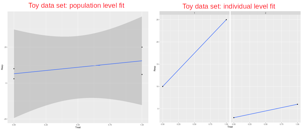
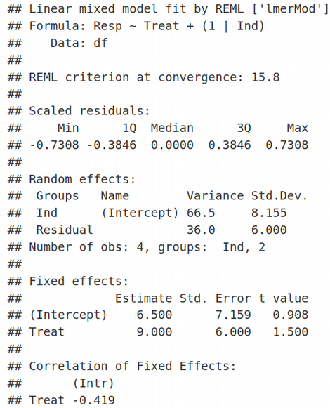
We use LMM when there is a non-independence between observations. In our case, the observations cluster within individuals. Let us apply LMM with Fixed Effects for slopes and intercepts and Random Effects for intercepts, this will result in adding a (1 | Ind) term to the Resp ~ Treat formula:
當觀測值之間存在非獨立性時,我們使用LMM。 在我們的案例中,觀察結果聚集在個人內部。 讓我們將LMM與“固定效應”應用于斜率和截距,將“ 隨機效應”應用于截距 ,這將導致在Resp?Treat公式中添加(1 | Ind)項:
Here REML=FALSE simply means that we are using the traditional Maximum Likelihood (ML) optimization and not Restricted Maximum Likelihood (we will talk about REML another time). In the Random Effects section of the lmer output, we see estimates for 2 parameters of minimization: residual variance corresponding to the standard deviation (Std.Dev.) of 4.243, and the random effects (shared between individuals) variance associated with the Intercept with the standard deviation of 5.766. Similarly, in the Fixed Effects section of the lmer output we can see two estimates for: 1) Intercept equal to 6.5, and 2) Slope / Treat equal to 9. Therefore, we have 4 parameters of optimization that correspond to 4 data points. The values of Fixed Effects make sense if we look at the very first figure in the Toy Data Set section and realize that the mean of two values for untreated samples is (3 + 10) / 2 =6.5, we will denote it as β1, and the mean of treated samples is (6 + 25) / 2 = 15.5, let us denote it as β2. The latter would be equivalent to 6.5 + 9, i.e. the estimate for the Fixed Effect of Intercept (=6.5) plus the estimate for the Fixed Effect of Slope (=9). Here, we pay attention to the exact values of Random and Fixed effects because we are going to reproduce them later when deriving and coding LMM.
這里REML = FALSE只是意味著我們使用的是傳統的最大似然(ML)優化,而不是受限的最大似然 (我們將在下一次討論REML)。 在lmer輸出的“隨機效應”部分中,我們看到了兩個最小化參數的估計值:與4.243的標準偏差(Std.Dev。)相對應的剩余方差 ,以及與截距相關的隨機效應(在個體之間共享)方差標準偏差為5.766。 同樣,在lmer輸出的“固定效果”部分中,我們可以看到兩個估計值:1)截距等于6.5,和2)斜率/對待等于9。因此,我們有4個優化參數對應于4個數據點。 如果我們看一下“玩具數據集”部分的第一個數字,并且意識到未處理的樣本的兩個值的平均值為(3 + 10)/ 2 = 6.5,則固定效果的值就有意義,我們將其表示為β1 ,并且處理后樣本的平均值為(6 + 25)/ 2 = 15.5,我們將其表示為β2 。 后者等于6.5 + 9,即截距固定效應的估計值(= 6.5)加上坡度固定效應的估計值(= 9)。 在這里,我們注意隨機和固定效果的確切值 ,因為稍后將在派生和編碼LMM時重現它們。
By default, lme4 R package and lmer R function do not provide measures of statistical significance such as p-values, however if you still would like to have a p-value of your LMM fit, it is possible to use lme function from the nlme R package:
默認情況下, lme4 R包和lmer R函數不提供統計意義的度量 ,例如p值,但是,如果您仍然希望LMM擬合的p值 ,則可以使用nlme中的 lme函數R包:
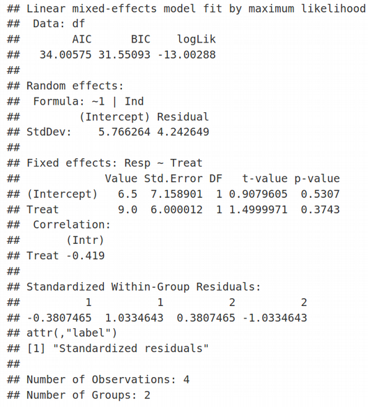
Again, here we have Random Effects for Intercept (StdDev = 5.766264) and Residual (StdDev = 4.242649), and Fixed Effects for Intercept (Value = 6.5) and Slope / Treat (Value = 9). Quite interesting, the standard errors of Fixed Effects and hence their t-values (t-value=1.5 for Treat) do not agree between lmer and lme. However, if we demand REML=TRUE in the lmer function, the Fixed Effects statistics including t-values are identical between lme and lmer, however the Random Effects statistics are different.
再次,這里我們具有截取的隨機效應( StdDev = 5.766264 )和殘差( StdDev = 4.242649 ),以及截距的固定效應(值= 6.5)和斜率/治療(值= 9)。 非常有趣的是,固定效應的標準誤差及其t值(“治療”的t值= 1.5)在lmer和lme之間不一致。 但是,如果我們在lmer函數中要求REML = TRUE,則lme和lmer之間的固定效應統計量(包括t值)是相同的 ,但是隨機效應統計量卻不同。
This is the difference between the Maximum Likelihood (ML) and Restricted Maximum Likelihood (REML) approaches that we will cover next time.
這是下一次我們將討論的最大可能性(ML)和受限最大可能性(REML)方法之間的差異。
LMM和配對T檢驗之間的關系 (Relation Between LMM and Paired T-Test)
Previously, we said that LMM is a more complex form of a simple paired t-test. Let us demonstrate that for our toy data set they do give identical outputs. On the way, we will also understand the technical difference between paired and un-paired t-tests. Let us first run the paired t-test between the treated and un-treated groups of samples taking into account the non-independence between them:
之前,我們說過LMM是簡單配對t檢驗的更復雜形式。 讓我們證明,對于我們的玩具數據集,它們確實提供了相同的輸出。 在途中,我們還將了解配對和非配對t檢驗之間的技術差異。 考慮到樣本之間的非獨立性,讓我們首先在已處理樣本組和未處理樣本組之間進行配對t檢驗:
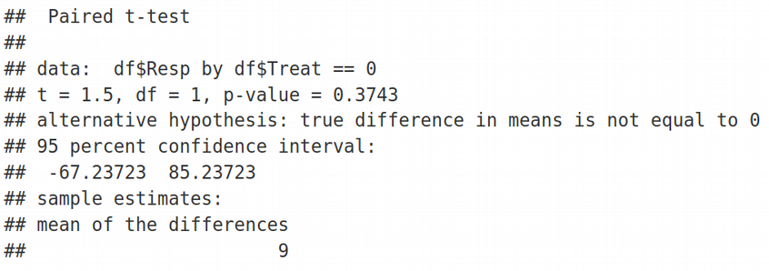
We can see that the t-value=1.5 and p-value = 0.3743 reported by the paired t-test are identical to the ones obtained by LMM using the nlme function or lmer with REML = TRUE. The reported by the paired t-test statistic “mean of the differences = 9” also agrees with the Fixed Effect estimates from lmer and nlme, remember we had the Treat Estimate = 9 that was simply the difference between the means of the treated and untreated samples.
我們可以看到,配對t檢驗報告的t值= 1.5和p值= 0.3743 與LMM使用nlme函數或lmer的REML = TRUE獲得的值相同。 配對t檢驗統計數據所報告的“差異均值= 9”也與lmer和nlme的“固定效應”估算值一致,請記住,我們的“治療估算值” = 9,這僅僅是治療與未治療方法之間的差異樣品。
Now, what is the paired t-test exactly doing? Well, the idea of the paired t-test is to make the setup look like a one-sample t-test where values in one group are tested for significant deviation from zero, which is a sort of the mean of the second group. In other words, we can view a paired t-test as if we shift the intercepts of the individual fits (see the very first figure) or the mean values of the untreated group down to zero. In a simple way, this would be equivalent to subtracting untreated Resp values from the treated ones, i.e. transforming the Resp variable to Resp_std (standardized Response) as shown below, and then performing an un-paired t-test on the Resp_std variable instead of Resp:
現在,配對t檢驗到底在做什么? 好吧,配對t檢驗的想法是使設置看起來像一個單樣本t檢驗 ,其中一組中的值被測試是否與零顯著偏離 ,這是第二組的平均值。 換句話說,我們可以查看成對的t檢驗,就好像我們將各個擬合的截距(參見第一個數字)或未處理組的平均值減小到零一樣 。 以一種簡單的方式,這等效于從已處理的值中減去未處理的Resp值,即如下所示將Resp變量轉換為Resp_std (標準響應),然后對Resp_std變量執行未配對的t檢驗,而不是響應:
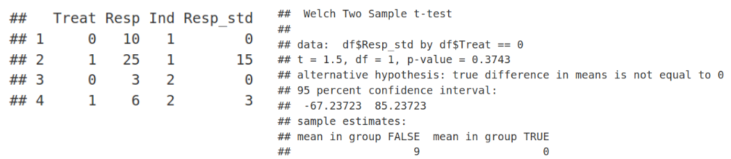
We observe that the values of Response became 0 for Treat = 0, i.e. untreated group, while the Response values of the treated group (Treat=1) are reduced by the values of the untreated group. Then we simply used the new Resp_std variable and ran an un-paired t-test, the result is equivalent to running paired t-test on the original Resp variable. Therefore, we can summarize that LMM reproduces the result of the paired t-test but allows for much more flexibility, for example, not only two (like for t-test) but multiple groups comparison etc.
我們觀察到,對于Treat = 0(即未治療組),Response的值變為0,而治療組(Treat = 1)的Response值減少了未經治療組的值。 然后,我們只需使用新的Resp_std變量并運行未配對的t檢驗,結果就相當于在原始Resp變量上運行配對的t檢驗。 因此,我們可以總結出,LMM再現了配對t檢驗的結果,但是允許更大的靈活性,例如,不僅兩個(像t檢驗一樣),而且可以進行多組比較等。
線性混合模型背后的數學 (Math Behind Linear Mixed Model)
Let us now try to derive a few LMM equations using our toy data set. We will again have a look at the 4 data points and make some mathematical notations accounting for treatment effects, β, which is nothing else than Fixed Effects, and the block-wise structure u due to points clustering within two individuals, which is actually the Random Effects contribution. We are going to express the Response (Resp) coordinates y in terms of β and u parameters.
現在讓我們嘗試使用玩具數據集導出一些LMM方程 。 我們將再次看看4個數據點,并提出一些數學符號占治療效果,β,這只不過是固定效應一樣 ,并逐塊結構U由于分兩個個體內成簇, 而這 實際上 是 隨機效應貢獻 。 我們將根據β和u參數來表示響應(Resp)坐標y 。
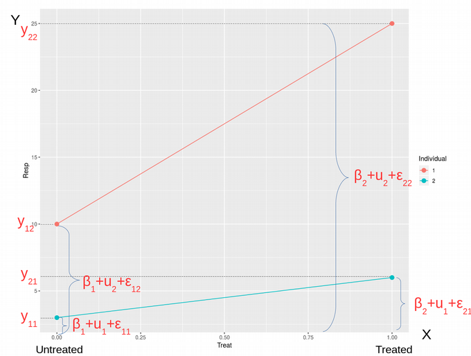
Here, β1 is the Response of the individuals in the Untreated state, while β2 is the Response on the Treatment. One can also say, that β1 is the mean of the untreated samples while β2 is the mean of the treated samples. The variables u1 and u2 are block variables accounting for effects specific to Individual #1 and Individual #2, respectively. Finally, ?ij ~ N(0, σ2) is the Residual error, i.e. the error we can’t model and can only try to minimize it as the goal of the Maximum Likelihood optimization problem. Therefore, we can write down the Response variable y as a combination of parameters β, u, i.e. Fixed and Random Effects, and ? as Eq. (1). In a general form, this system of algebraic equations can be rewritten as Eq. (2), where the index i = 1, 2 corresponds to treatment effects and j = 1, 2 describes individual effects. We can also express this system of equations in the matrix form Eq. (3). Therefore we arrive to the following famous matrix form of LMM which is shown in all textbooks but not always properly explained, Eq. (4).
在此, β1是未治療狀態的個體的React,而β2是對治療的React 。 也可以說, β1是未處理樣品的平均值,而β2是已處理樣品的平均值。 變量u1和u2是塊變量,分別說明特定于個人#1和個人#2的影響。 最后, ?ij?N(0,σ2)是殘差誤差 ,即我們無法建模的誤差,只能將其最小化作為最大似然優化問題的目標。 因此,我們可以將Response變量y記為參數 β , u的組合 ,即固定 效應和隨機效應 ,以及? 如式 (1)。 通常,該代數方程組可以重寫為等式。 (2),其中索引i = 1、2對應于治療效果,而j = 1、2描述單個效果。 我們還可以以矩陣形式Eq表示此方程組。 (3)。 因此,我們得出以下著名的LMM矩陣形式,該形式在所有教科書中均已顯示,但并非總是正確解釋。 (4)。
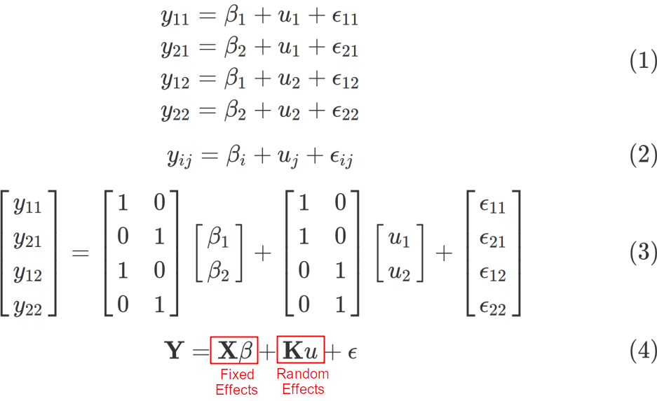
Here, X is called the design matrix and K is called the block matrix, it codes the relationship between the data points, i.e. whether they come from related individuals or even from the same individual like in our case. It is important to note that the treatment is modeled as a fixed effect because the levels treated-untreated exhaust all possible outcomes of treatment. In contrast, the block-wise structure of the data is modeled as a Random Effect since the individuals were sampled from population, and might not correctly represent the entire population of individuals. In other words, there is an error associated with the random effects, i.e. uj ~ N(0, σs2), while fixed affects are assumed to be error free. For example, sex is usually modeled as a Fixed Effect because it is usually assumed to have only two levels (males, females), while batch-effects in Life Sciences should be modeled as Random Effects because potentially additional experimental protocols or labs would produce many more, that is many levels, systematic differences between samples that confound the data analysis. As a rule of thumb one could think that Fixed Effects should not have many levels, while Random Effects are typically multi-level categorical variables where the levels represent just a sample of all possibilities but not all of them.
在這里, X稱為設計矩陣 , K稱為塊矩陣 ,它對數據點之間的關系進行編碼,即數據點是來自相關個人,還是像我們一樣來自同一個人。 重要的是要注意,將治療建模為固定效果,因為未經處理的水平會耗盡所有可能的治療結果。 相比之下,數據的逐塊結構被建模為隨機效應,因為個體是從總體中采樣的 ,因此可能無法正確代表整個個體。 換句話說,存在與隨機效應相關的誤差,即uj?N(0,σs2) ,而固定效應則假定為無誤差。 例如,通常將性別建模為固定效應,因為通常假定性別只有兩個級別(男性,女性) ,而生命科學中的批量效應應建模為隨機效應,因為可能會通過其他實驗方案或實驗室產生很多效應更重要的是,樣本之間存在許多層次上的系統差異,這混淆了數據分析。 根據經驗,固定效應不應有多個級別,而隨機效應通常是多級類別變量,其中級別僅代表所有可能性的樣本,但并不代表所有可能性。
Let us proceed with deriving the mean and the variance of the data points Y. Since both the Random Effect error and the Residual error come from Normal distribution with zero mean, while the non-zero component in E[Y] originates from the Fixed Effect, we can express the expected value of Y as Eq. (5). Next, the variance of the Fixed Effect term is zero, as Fixed Effects are assumed to be error free, therefore, for the variance of Y we obtain Eq. (6).
讓我們繼續推導數據點 Y的均值和方差 。 由于隨機效應誤差和殘余誤差均來自均值為零的正態分布,而E [ Y ]中的非零分量源自固定效應,因此我們可以將Y的期望值表示為Eq。 (5)。 接下來,固定效果項的方差為零,因為固定效果被假定為無誤差,因此,對于Y的方差,我們得到等式。 (6)。
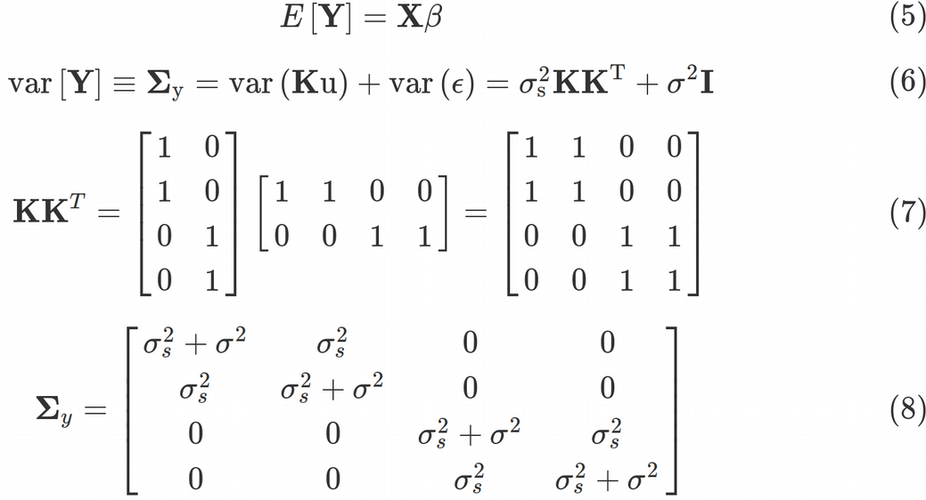
Eq. (6) was obtained by taking into account that var(Ku)=K*var(u)*K^T and var(?) = σ2*I and var(u)= σs2*I, where I is a 4 x 4 identity matrix. Here, σ2 is the Residual variance (unmodeled/unreduced error), and σs2 is the random Intercept effects (shared across data points) variance. The matrix in front of σs2 is called the kinship matrix and is given by Eq. (7). The kinship matrix codes all relatedness between data points. For example, some data points may come from genetically related people, geographic locations in close proximity, some data points may come from technical replicates. Those relationships are coded in the kinship matrix. Thus, the variance-covariance matrix of the data points from Eq. (6) takes the ultimate form of Eq. (8). Once we have obtained the variance-covariance matrix, we can continue with optimization procedure of the Maximum Likelihood function that requires the variance-covariance.
等式 (6)通過考慮到變種(K U)= K *變種(U)* K ^ T和VAR(ε)=σ2* I和變種(U)=σ秒2* I,其中I是獲得一個4 x 4的單位矩陣 。 這里,σ是2 殘余方差 (未建模/未還原的錯誤),以及強度σs2是隨機攔截效果(跨數據點共享)方差 。 σs2前面的矩陣稱為親屬矩陣 ,由等式給出。 (7)。 親屬關系矩陣編碼數據點之間的所有相關性。 例如,某些數據點可能來自與遺傳相關的人,地理位置非常接近,某些數據點可能來自技術復制。 這些關系在親屬關系矩陣中編碼。 因此,來自等式的數據點的方差-協方差矩陣。 (6)采用等式的最終形式。 (8)。 一旦獲得方差-協方差矩陣,我們就可以繼續進行需要方差-協方差的最大似然函數的優化過程。
LMM來自最大似然(ML)原理 (LMM from Maximum Likelihood (ML) Principle)
Why did we spend so much time deriving the variance-covariance matrix and what does it have to do with the linear regression? It turns out that the whole concept of fitting a linear model, as well as many other if not all concepts of traditional Frequentist statistics, comes from the Maximum Likelihood (ML) principle. For this purpose, we need to maximize the Multivariate Gaussian distribution function with respect to parameters β1, β2, σs2 and σ2, Eq. (9).
為什么我們要花費大量時間來得出方差-協方差矩陣,它與線性回歸有什么關系? 事實證明, 擬合線性模型的整個概念以及傳統頻率統計的許多其他(如果不是全部)概念都來自最大似然(ML) 原理 。 為此,我們需要針對參數β1 , β2 , σs2和σ2 ,等式最大化多元高斯 分布函數 。 (9)。
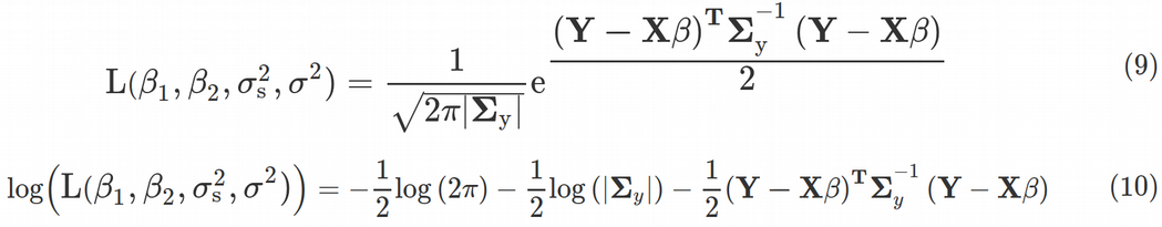
Here |Σy| denotes the determinant of the variance-covariance matrix. We see that the inverse matrix and determinant of the variance-covariance matrix are explicitly included into the Likelihood function, this is why we had to compute its expression via the random effects variance σs2 and residual variance σ2. Maximization of the Likelihood function is equivalent to minimization of the log-likelihood function, Eq. (10).
在這里 ΣY | 表示方差-協方差矩陣的行列式。 我們看到方差-協方差矩陣的逆矩陣和行列式明確包含在似然函數中,這就是為什么我們必須通過隨機效應方差 σs2和殘差方差 σ2計算其表達式的原因。 似然函數的最大化等效于對數似然函數 Eq的最小化 。 (10)。
We will need to perform a tedious symbolic derivation of the determinant of the variance-covariance matrix, the inverse variance-covariance matrix and the product of the inverse variance-covariance matrix with Y?Xβ terms. To my experience, this is hard to do in R / Python, however we can use Maple (or similarly Mathematica or Matlab) for making symbolic calculations, and derive the expressions for determinant and inverse of the variance-covariance matrix:
我們將需要對方差-協方差矩陣, 逆方差-協方差矩陣和具有Y - Xβ 項的 方差-協方差矩陣的乘積執行繁瑣的符號推導 。 以我的經驗,這在R / Python中很難做到,但是我們可以使用Maple (或類似的 Mathematica 或 Matlab )進行符號計算,并導出方差-協方差矩陣的行列式和逆式的表達式:
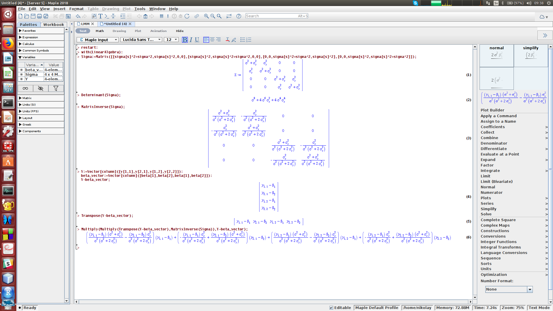
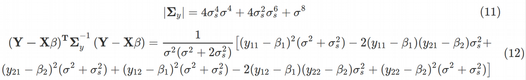
Using Maple we can obtain the determinant of the variance-covariance matrix as Eq. (11). Next, the last term in Eq. (10) for log-likelihood takes the form of Eq. (12).
使用Maple,我們可以獲得方差-協方差矩陣的行列式。 (11)。 接下來,等式中的最后一項。 (10)對數似然采用等式的形式。 (12)。
Now we are ready to perform the numeric minimization of the log-likelihood function with respect to β1, β2, σs2 and σ2 using the optim R function:
現在,我們準備使用優化 R函數對β1 , β2 , σs2和σ2執行對數似然函數的數值最小化:
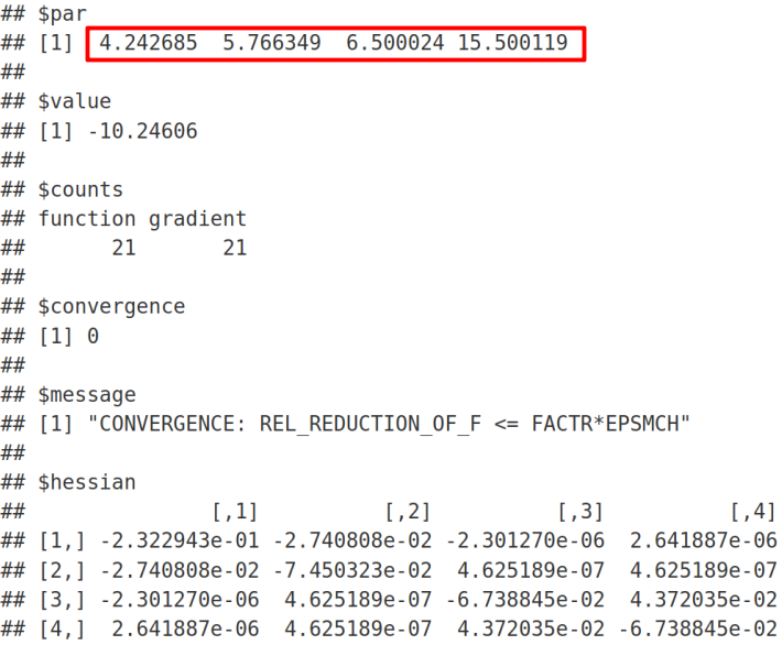
We can see that the minimization algorithm has successfully converged since we got the “convergence = 0” message. In the output, σ=4.242640687 is the residual standard deviation, which exactly reproduces the result from lme and lmer (with REML = FALSE). By analogy, σs=5.766281297 is the shared standard deviation that again exactly reproduces the corresponding Random Effects Intercept outputs from lme and lmer (with REML = FALSE) functions. As expected, the Fixed Effect β1 = 6.5 is the mean of the untreated samples in agreement with the Intercept Fixed Effect Estimate from lmer and lme. Next, β2 = 15.5 is the mean of treated samples, which is the Intercept Fixed Effect Estimate (= 6.5) plus the Slope / Treat Fixed Effect Estimate (= 9) from lmer and lme R functions.
我們可以看到,自從收到“ convergence = 0”消息以來,最小化算法已成功收斂 。 在輸出中, σ= 4.242640687是殘余標準偏差 ,它精確地再現了 lme和lmer 的結果 (REML = FALSE)。 以此類推, σs= 5.766281297是共享的標準偏差 ,該偏差再次精確地再現了來自lme和lmer(具有REML = FALSE)功能的相應的“隨機效果攔截”輸出。 正如預期的那樣,固定效應β1= 6.5的平均值與固定效應估算和11聚物倫敦金屬交易所攔截協議未經處理的樣品。 接下來, β2= 15.5是已處理樣品的平均值,它是截距固定效果估計值(= 6.5)加上來自lmer和lme R函數的斜率/處理固定效果估計值(= 9)。
Fantastic job! We have successfully reproduced the Fixed Effects and Random Effects outputs from lmer / lme functions by deriving and coding the Linear Mixed Model (LMM) from scratch!
很棒的工作! 通過從頭開始推導和編碼線性混合模型(LMM),我們已經成功地從lmer / lme函數復制了固定效果和隨機效果輸出!
摘要 (Summary)
In this article, we have learnt how to derive and code a Linear Mixed Model (LMM) with Fixed and Random Effects on a toy data set. We covered the relation between LMM and the paired t-test, and reproduced the Fixed and Random Effects parameters from lmer and lme R functions.
在本文中,我們學習了如何在 玩具數據集 上導出具有 固定和隨機效應的線性混合模型(LMM)并進行編碼。 我們介紹了LMM和配對t檢驗之間的關系,并從lmer和lme R函數復制了“固定效應”和“隨機效應”參數。
In the comments below, let me know which analytical techniques from Life Sciences seem especially mysterious to you and I will try to cover them in the future posts. Check the codes from the post on my Github. Follow me at Medium Nikolay Oskolkov, in Twitter @NikolayOskolkov and do connect in Linkedin. In the next post, we are going to cover the difference between the Maximum Likelihood (ML) and Restricted Maximum Likelihood (REML) approaches, stay tuned.
在下面的評論中,讓我知道生命科學的哪些分析技術對您來說似乎特別神秘 ,我將在以后的文章中嘗試介紹它們。 在我的Github上檢查帖子中的代碼。 跟隨我在中型Nikolay Oskolkov,在Twitter @NikolayOskolkov上進行連接,并在Linkedin中進行連接。 在下一篇文章中,我們將介紹 請密切關注最大可能性(ML)和限制最大可能性(REML)方法之間的差異。
翻譯自: https://towardsdatascience.com/linear-mixed-model-from-scratch-f29b2e45f0a4
一般線性模型和混合線性模型
本文來自互聯網用戶投稿,該文觀點僅代表作者本人,不代表本站立場。本站僅提供信息存儲空間服務,不擁有所有權,不承擔相關法律責任。 如若轉載,請注明出處:http://www.pswp.cn/news/388424.shtml 繁體地址,請注明出處:http://hk.pswp.cn/news/388424.shtml 英文地址,請注明出處:http://en.pswp.cn/news/388424.shtml
如若內容造成侵權/違法違規/事實不符,請聯系多彩編程網進行投訴反饋email:809451989@qq.com,一經查實,立即刪除!相關文章

《企業私有云建設指南》-導讀

vs2005的webbrowser控件如何接收鼠標事件
![[TimLinux] Python 迭代器(iterator)和生成器(generator)](http://pic.xiahunao.cn/[TimLinux] Python 迭代器(iterator)和生成器(generator))
[TimLinux] Python 迭代器(iterator)和生成器(generator)

太原冶金技師學院計算機系,山西冶金技師學院專業都有什么

海南首例供港造血干細胞志愿者啟程赴廣東捐獻

如何擊敗Python的問題

KindEditor解決上傳視頻不能在手機端顯示的問題

湖北經濟學院的計算機是否強,graphics-ch11-真實感圖形繪制_湖北經濟學院:計算機圖形學_ppt_大學課件預覽_高等教育資訊網...

ARP攻擊網絡上不去,可以進行mac地址綁定

《獨家記憶》見面會高甜寵粉 張超現場解鎖隱藏技能

計算機軟件技術基礎fifo算法,軟件技術基礎真題
)
NOI 2016 優秀的拆分 (后綴數組+差分)

多元線性回歸 python_Python中的多元線性回歸

關于apache和tomcat集群,線程是否占用實驗

爬蟲之數據解析的三種方式

相對于硬件計算機軟件就是,計算機的軟件是將解決問題的方法,軟件是相對于硬件來說的...

數據冒險控制冒險_勞動生產率和其他冒險

如何把一個java程序打包成exe文件,運行在沒有java虛

Java后端WebSocket的Tomcat實現
