深度學習 Day10——T10數據增強

🍨 本文為🔗365天深度學習訓練營中的學習記錄博客
🍖 原作者：K同學啊 | 接輔導、項目定制

文章目錄

前言
一、我的環境
二、代碼實現與執行結果
- 1.引入庫
- 2.設置GPU（如果使用的是CPU可以忽略這步）
- 3.導入數據
- 4.查看數據
- 5.加載數據
- 6.再次檢查數據
- 7.配置數據集
- 8.可視化數據
- 9.構建CNN網絡模型
- 10.編譯模型
- 11.訓練模型
- 12.模型評估
三、知識點詳解
- 1.圖像增強
- 1.1TensorFlow 之中進行圖像數據增強
- - 1.1.1使用 tf.keras 的預處理層進行圖像數據增強
  - 1.1.2 使用 tf.image 進行數據增強
- 1.2自定義增強函數
- 1.3 圖像增強數據與原始數據合并作為新樣本
總結

前言

本文將采用CNN實現貓狗識別。簡單講述實現代碼與執行結果，并淺談涉及知識點。
關鍵字：圖像增強

一、我的環境

電腦系統：Windows 11
語言環境：python 3.8.6
編譯器：pycharm2020.2.3
深度學習環境：TensorFlow 2.10.1
顯卡：NVIDIA GeForce RTX 4070

二、代碼實現與執行結果

1.引入庫

from PIL import Image
import numpy as np
from pathlib import Path
import tensorflow as tf
from tensorflow.keras import datasets, layers, models, regularizers
from tensorflow.keras.callbacks import ModelCheckpoint, EarlyStopping
from tensorflow.keras.applications.vgg16 import VGG16
from tensorflow.keras import layers, models, Input
from tensorflow.keras.models import Model
from tensorflow.keras.layers import Conv2D, MaxPooling2D, Dense, Flatten, Dropout, BatchNormalization
from tqdm import tqdm
import tensorflow.keras.backend as K
import matplotlib.pyplot as plt
import warningswarnings.filterwarnings('ignore')  # 忽略一些warning內容，無需打印

2.設置GPU（如果使用的是CPU可以忽略這步）

'''前期工作-設置GPU（如果使用的是CPU可以忽略這步）'''
# 檢查GPU是否可用
print(tf.test.is_built_with_cuda())
gpus = tf.config.list_physical_devices("GPU")
print(gpus)
if gpus:gpu0 = gpus[0]  # 如果有多個GPU，僅使用第0個GPUtf.config.experimental.set_memory_growth(gpu0, True)  # 設置GPU顯存用量按需使用tf.config.set_visible_devices([gpu0], "GPU")

執行結果

True
[PhysicalDevice(name='/physical_device:GPU:0', device_type='GPU')]

3.導入數據

數據鏈接: 貓狗數據

'''前期工作-導入數據'''
data_dir = r"D:\DeepLearning\data\CatDog"
data_dir = Path(data_dir)

4.查看數據

'''前期工作-查看數據'''
image_count = len(list(data_dir.glob('*/*.png')))
print("圖片總數為：", image_count)
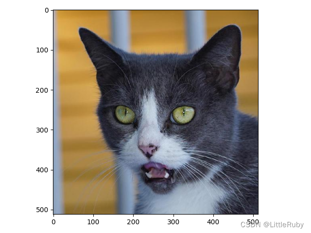
image_list = list(data_dir.glob('cat/*.png'))
image = Image.open(str(image_list[1]))
# 查看圖像實例的屬性
print(image.format, image.size, image.mode)
plt.imshow(image)
plt.show()

執行結果：

圖片總數為： 3400
JPEG (512, 512) RGB

在這里插入圖片描述

5.加載數據

 '''數據預處理-加載數據'''
batch_size = 64
img_height = 224
img_width = 224
"""
關于image_dataset_from_directory()的詳細介紹可以參考文章：https://mtyjkh.blog.csdn.net/article/details/117018789
"""
train_ds = tf.keras.preprocessing.image_dataset_from_directory(data_dir,validation_split=0.2,subset="training",seed=12,image_size=(img_height, img_width),batch_size=batch_size)
val_ds = tf.keras.preprocessing.image_dataset_from_directory(data_dir,validation_split=0.2,subset="validation",seed=12,image_size=(img_height, img_width),batch_size=batch_size)
# 我們可以通過class_names輸出數據集的標簽。標簽將按字母順序對應于目錄名稱。
class_names = train_ds.class_names
print(class_names)

運行結果：

Found 3400 files belonging to 2 classes.
Using 2720 files for training.
Found 3400 files belonging to 2 classes.
Using 680 files for validation.
['cat', 'dog']

6.再次檢查數據

'''數據預處理-再次檢查數據'''
# Image_batch是形狀的張量（32,180,180,3）。這是一批形狀180x180x3的32張圖片（最后一維指的是彩色通道RGB）。
# Label_batch是形狀（32，）的張量，這些標簽對應32張圖片
for image_batch, labels_batch in train_ds:print(image_batch.shape)print(labels_batch.shape)break

運行結果

(64, 224, 224, 3)
(64,)

7.配置數據集

AUTOTUNE = tf.data.AUTOTUNEdef preprocess_image(image, label):return (image / 255.0, label)# 歸一化處理
train_ds = train_ds.map(preprocess_image, num_parallel_calls=AUTOTUNE)
val_ds = val_ds.map(preprocess_image, num_parallel_calls=AUTOTUNE)
test_ds = test_ds.map(preprocess_image, num_parallel_calls=AUTOTUNE)train_ds = train_ds.cache().shuffle(1000).prefetch(buffer_size=AUTOTUNE)
val_ds = val_ds.cache().prefetch(buffer_size=AUTOTUNE)

8.可視化數據

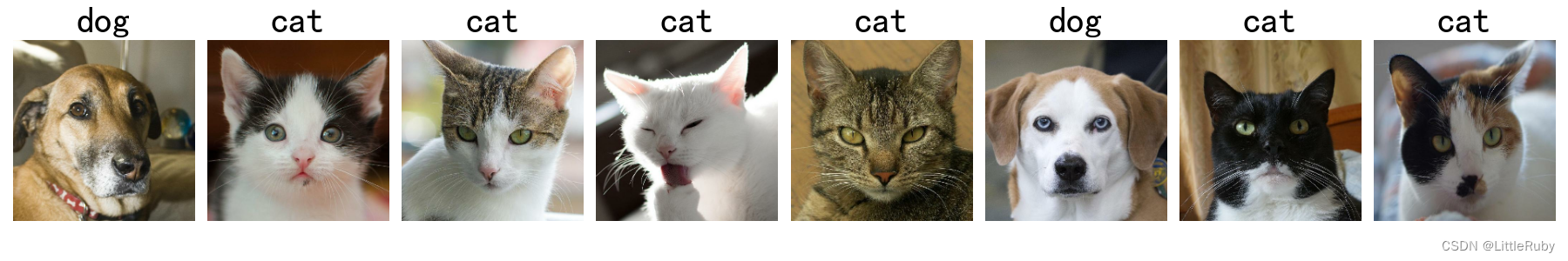
'''數據預處理-可視化數據'''
plt.figure(figsize=(18, 3))
for images, labels in train_ds.take(2):for i in range(8):ax = plt.subplot(1, 8, i + 1)plt.imshow(images[i].numpy().astype("uint8"))plt.title(class_names[labels[i]], fontsize=40)plt.axis("off")
# 顯示圖片
plt.show()

在這里插入圖片描述

9.構建CNN網絡模型

#VGG16
def VGG16(class_names, img_height, img_width):model = models.Sequential([# 1layers.Conv2D(filters=64, kernel_size=(3, 3), activation='relu', padding='same',input_shape=(img_height, img_width, 3)),layers.Conv2D(filters=64, kernel_size=(3, 3), activation='relu', padding='same'),layers.MaxPool2D(pool_size=(2, 2), strides=2),# 2layers.Conv2D(filters=128, kernel_size=(3, 3), activation='relu', padding='same'),layers.Conv2D(filters=128, kernel_size=(3, 3), activation='relu', padding='same'),layers.MaxPool2D(pool_size=(2, 2), strides=2),# 3layers.Conv2D(filters=256, kernel_size=(3, 3), activation='relu', padding='same'),layers.Conv2D(filters=256, kernel_size=(3, 3), activation='relu', padding='same'),layers.Conv2D(filters=256, kernel_size=(3, 3), activation='relu', padding='same'),layers.MaxPool2D(pool_size=(2, 2), strides=2),# 4layers.Conv2D(filters=512, kernel_size=(3, 3), activation='relu', padding='same'),layers.Conv2D(filters=512, kernel_size=(3, 3), activation='relu', padding='same'),layers.Conv2D(filters=512, kernel_size=(3, 3), activation='relu', padding='same'),layers.MaxPool2D(pool_size=(2, 2), strides=2),# 5layers.Conv2D(filters=512, kernel_size=(3, 3), activation='relu', padding='same'),layers.Conv2D(filters=512, kernel_size=(3, 3), activation='relu', padding='same'),layers.Conv2D(filters=512, kernel_size=(3, 3), activation='relu', padding='same'),layers.MaxPool2D(pool_size=(2, 2), strides=2),# FClayers.Flatten(),layers.Dense(4096, activation='relu'),layers.Dense(4096, activation='relu'),layers.Dense(len(class_names), activation='softmax')])return model
model = VGG16(class_names, img_height, img_width)
model.summary()

網絡結構結果如下：

Model: "sequential_1"
_________________________________________________________________Layer (type)                Output Shape              Param #   
=================================================================conv2d (Conv2D)             (None, 224, 224, 64)      1792      conv2d_1 (Conv2D)           (None, 224, 224, 64)      36928     max_pooling2d (MaxPooling2D  (None, 112, 112, 64)     0         )                                                               conv2d_2 (Conv2D)           (None, 112, 112, 128)     73856     conv2d_3 (Conv2D)           (None, 112, 112, 128)     147584    max_pooling2d_1 (MaxPooling  (None, 56, 56, 128)      0         2D)                                                             conv2d_4 (Conv2D)           (None, 56, 56, 256)       295168    conv2d_5 (Conv2D)           (None, 56, 56, 256)       590080    conv2d_6 (Conv2D)           (None, 56, 56, 256)       590080    max_pooling2d_2 (MaxPooling  (None, 28, 28, 256)      0         2D)                                                             conv2d_7 (Conv2D)           (None, 28, 28, 512)       1180160   conv2d_8 (Conv2D)           (None, 28, 28, 512)       2359808   conv2d_9 (Conv2D)           (None, 28, 28, 512)       2359808   max_pooling2d_3 (MaxPooling  (None, 14, 14, 512)      0         2D)                                                             conv2d_10 (Conv2D)          (None, 14, 14, 512)       2359808   conv2d_11 (Conv2D)          (None, 14, 14, 512)       2359808   conv2d_12 (Conv2D)          (None, 14, 14, 512)       2359808   max_pooling2d_4 (MaxPooling  (None, 7, 7, 512)        0         2D)                                                             flatten (Flatten)           (None, 25088)             0         dense (Dense)               (None, 4096)              102764544 dense_1 (Dense)             (None, 4096)              16781312  dense_2 (Dense)             (None, 2)                 8194      =================================================================
Total params: 134,268,738
Trainable params: 134,268,738
Non-trainable params: 0
_________________________________________________________________

10.編譯模型

'''編譯模型'''
#設置初始學習率
initial_learning_rate = 1e-4
opt = tf.keras.optimizers.Adam(learning_rate=initial_learning_rate)
model.compile(optimizer=opt,loss='sparse_categorical_crossentropy',metrics=['accuracy'])

11.訓練模型

'''訓練模型'''
epochs = 10
history = model.fit(train_ds,validation_data=val_ds,epochs=epochs,shuffle=False
)

訓練記錄如下：

Epoch 1/1043/43 [==============================] - 42s 606ms/step - loss: 0.6830 - accuracy: 0.5511 - val_loss: 0.7328 - val_accuracy: 0.6630
Epoch 2/10
43/43 [==============================] - 17s 384ms/step - loss: 0.4927 - accuracy: 0.7614 - val_loss: 0.3283 - val_accuracy: 0.8714
Epoch 3/10
43/43 [==============================] - 17s 385ms/step - loss: 0.2113 - accuracy: 0.9165 - val_loss: 0.1986 - val_accuracy: 0.9221
Epoch 4/10
43/43 [==============================] - 17s 385ms/step - loss: 0.1173 - accuracy: 0.9555 - val_loss: 0.0977 - val_accuracy: 0.9620
Epoch 5/10
43/43 [==============================] - 17s 385ms/step - loss: 0.0561 - accuracy: 0.9798 - val_loss: 0.0789 - val_accuracy: 0.9728
Epoch 6/10
43/43 [==============================] - 17s 385ms/step - loss: 0.0483 - accuracy: 0.9816 - val_loss: 0.0578 - val_accuracy: 0.9783
Epoch 7/10
43/43 [==============================] - 17s 385ms/step - loss: 0.0457 - accuracy: 0.9838 - val_loss: 0.0551 - val_accuracy: 0.9783
Epoch 8/10
43/43 [==============================] - 17s 385ms/step - loss: 0.0372 - accuracy: 0.9875 - val_loss: 0.0985 - val_accuracy: 0.9692
Epoch 9/10
43/43 [==============================] - 17s 385ms/step - loss: 0.0324 - accuracy: 0.9915 - val_loss: 0.0264 - val_accuracy: 0.9873
Epoch 10/10
43/43 [==============================] - 17s 385ms/step - loss: 0.0109 - accuracy: 0.9967 - val_loss: 0.0408 - val_accuracy: 0.9891
2/2 [==============================] - 0s 116ms/step - loss: 0.0615 - accuracy: 0.9922
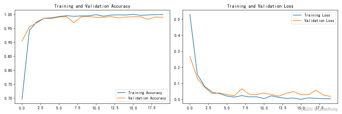
Accuracy 0.9921875

12.模型評估

'''模型評估'''
acc = history.history['accuracy']
val_acc = history.history['val_accuracy']
loss = history.history['loss']
val_loss = history.history['val_loss']
epochs_range = range(len(loss))
plt.figure(figsize=(12, 4))
plt.subplot(1, 2, 1)
plt.plot(epochs_range, acc, label='Training Accuracy')
plt.plot(epochs_range, val_acc, label='Validation Accuracy')
plt.legend(loc='lower right')
plt.title('Training and Validation Accuracy')
plt.subplot(1, 2, 2)
plt.plot(epochs_range, loss, label='Training Loss')
plt.plot(epochs_range, val_loss, label='Validation Loss')
plt.legend(loc='upper right')
plt.title('Training and Validation Loss')
plt.show()loss, acc = model.evaluate(test_ds)
print("Accuracy", acc)

執行結果
在這里插入圖片描述

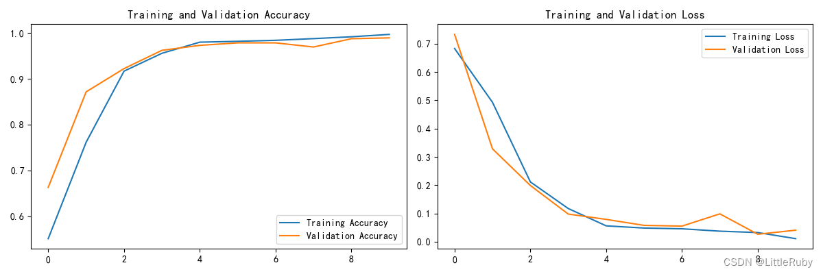
2/2 [==============================] - 0s 116ms/step - loss: 0.0615 - accuracy: 0.9922
Accuracy 0.9921875

三、知識點詳解

1.圖像增強

在深度學習中，有的時候訓練集不夠多，或者某一類數據較少，或者為了防止過擬合，讓模型更加魯棒性，data augmentation是一個不錯的選擇。
通過數據增強，我們可以將一些已經存在的數據進行相應的變換（可以選擇將這些變換之后的數據增加到新的原來的數據集之中，也可以直接在原來的數據集上進行變換），從而實現數據種類多樣性的增加。
對于圖片數據，常見的數據增強方式包括：

隨機水平翻轉：
隨機的裁剪；
隨機調整明亮程度；
其他方式等

1.1TensorFlow 之中進行圖像數據增強

在 TensorFlow 之中進行圖像數據增強的方式主要有兩種：

使用 tf.keras 的預處理層進行圖像數據增強；
使用 tf.image 進行數據增強。

1.1.1使用 tf.keras 的預處理層進行圖像數據增強

使用 tf.keras 的預處理層進行圖像數據增強要使用的最主要的 API 包括在一下包之中：

tf.keras.layers.experimental.preprocessing

在這個包之中，我們最常用的數據增強 API 包括：

tf.keras.layers.experimental.preprocessing.RandomFlip(mode): 將輸入的圖片進行隨機翻轉，一般我們會取 mode=“horizontal” ，因為這代表水平旋轉；而 mode=“vertical” 則代表隨機進行上下翻轉；
tf.keras.layers.experimental.preprocessing.RandomRotation§: 按照旋轉角度（單位為弧度） p 將輸入的圖片進行隨機的旋轉；
tf.keras.layers.experimental.preprocessing.RandomContrast§：按照 P 的概率將輸入的圖片進行隨機的圖像色相翻轉；
tf.keras.layers.experimental.preprocessing.CenterCrop(height, width)：使用 height * width 的大小的裁剪框，在數據的中心進行裁剪。
該API有兩種使用方式：一個是將其嵌入model中，一個是在Dataset數據集中進行數據增強

方式一：嵌入model中
調用方式如下

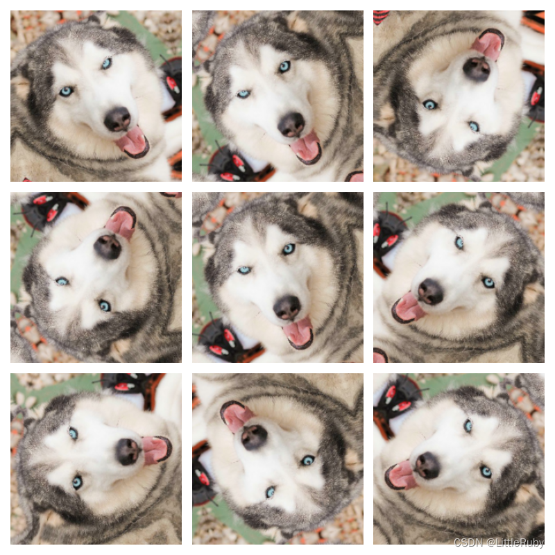
# tf.keras.layers.experimental.preprocessing圖像增強 第一個層表示進行隨機的水平和垂直翻轉，而第二個層表示按照 0.2 的弧度值進行隨機旋轉。
data_augmentation = tf.keras.Sequential([tf.keras.layers.experimental.preprocessing.RandomFlip("horizontal_and_vertical",input_shape=(img_height, img_width, 3)),tf.keras.layers.experimental.preprocessing.RandomRotation(0.2),
])
model = tf.keras.Sequential([data_augmentation,layers.Conv2D(16, 3, padding='same', activation='relu'),layers.MaxPooling2D(),
])
# 圖像增強 可視化效果圖
for images, labels in train_ds.take(1):# Add the image to a batch.image = tf.expand_dims(images[0], 0)plt.figure(figsize=(8, 8))for i in range(9):augmented_image = data_augmentation(image)ax = plt.subplot(3, 3, i + 1)plt.imshow(augmented_image[0])plt.axis("off")plt.show()break

本文案例使用如下

data_augmentation = tf.keras.Sequential([tf.keras.layers.experimental.preprocessing.RandomFlip("horizontal_and_vertical",input_shape=(img_height, img_width, 3)),tf.keras.layers.experimental.preprocessing.RandomRotation(0.2),
])
#方式一圖像增強：tf.keras.layers.experimental.preprocessing方式實現的圖像增強，嵌入模型中
#只有在模型訓練時（Model.fit）才會進行增強，在模型評估(Model.evaluate)以及預測(Model.predict)時并不會進行增強操作
def VGG16_aug0(class_names, img_height, img_width):model = models.Sequential([data_augmentation,# 1layers.Conv2D(filters=64, kernel_size=(3, 3), activation='relu', padding='same',input_shape=(img_height, img_width, 3)),layers.Conv2D(filters=64, kernel_size=(3, 3), activation='relu', padding='same'),layers.MaxPool2D(pool_size=(2, 2), strides=2),# 2layers.Conv2D(filters=128, kernel_size=(3, 3), activation='relu', padding='same'),layers.Conv2D(filters=128, kernel_size=(3, 3), activation='relu', padding='same'),layers.MaxPool2D(pool_size=(2, 2), strides=2),# 3layers.Conv2D(filters=256, kernel_size=(3, 3), activation='relu', padding='same'),layers.Conv2D(filters=256, kernel_size=(3, 3), activation='relu', padding='same'),layers.Conv2D(filters=256, kernel_size=(3, 3), activation='relu', padding='same'),layers.MaxPool2D(pool_size=(2, 2), strides=2),# 4layers.Conv2D(filters=512, kernel_size=(3, 3), activation='relu', padding='same'),layers.Conv2D(filters=512, kernel_size=(3, 3), activation='relu', padding='same'),layers.Conv2D(filters=512, kernel_size=(3, 3), activation='relu', padding='same'),layers.MaxPool2D(pool_size=(2, 2), strides=2),# 5layers.Conv2D(filters=512, kernel_size=(3, 3), activation='relu', padding='same'),layers.Conv2D(filters=512, kernel_size=(3, 3), activation='relu', padding='same'),layers.Conv2D(filters=512, kernel_size=(3, 3), activation='relu', padding='same'),layers.MaxPool2D(pool_size=(2, 2), strides=2),# FClayers.Flatten(),layers.Dense(4096, activation='relu'),layers.Dense(4096, activation='relu'),layers.Dense(len(class_names), activation='softmax')])return model
model = VGG16_aug0(class_names, img_height, img_width) # 方式一圖像增強
model.summary()# 圖像增強 可視化效果圖
for images, labels in train_ds.take(1):# Add the image to a batch.image = tf.expand_dims(images[0], 0)plt.figure(figsize=(8, 8))for i in range(9):augmented_image = data_augmentation(image)ax = plt.subplot(3, 3, i + 1)plt.imshow(augmented_image[0])plt.axis("off")plt.show()break

在這里插入圖片描述

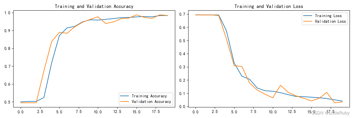
方式二：在Dataset數據集中進行數據增強
本文案例使用如下

#方式二圖像增強：tf.keras.layers.experimental.preprocessing方式實現的圖像增強.在Dataset數據集中進行數據增強
AUTOTUNE = tf.data.AUTOTUNEdef prepare(ds):ds = ds.map(lambda x, y: (data_augmentation(x, training=True), y), num_parallel_calls=AUTOTUNE)return ds
train_ds1 = prepare(train_ds)'''訓練模型'''
epochs = 20
history = model.fit(train_ds1,validation_data=val_ds,epochs=epochs    
)

在這里插入圖片描述
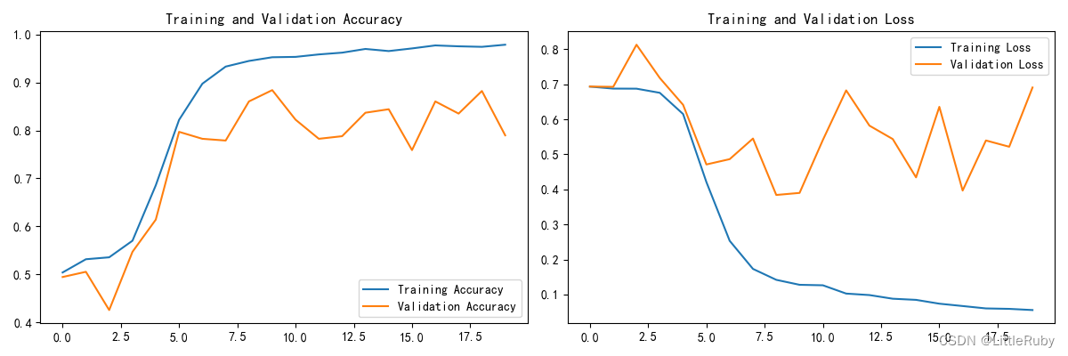
本文試驗效果并不理想

1.1.2 使用 tf.image 進行數據增強

使用 tf.image 是 TensorFlow 最原生的一種增強方式，使用這種方式可以實現更多、更加個性化的數據增強。

其中包含的數據增強方式主要包括：

tf.image.flip_left_right (img)：將圖片進行水平翻轉；
tf.image.rgb_to_grayscale (img)：將 RGB 圖像轉化為灰度圖像；
tf.image.adjust_saturation (image, f)：將 image 圖像按照 f 參數進行飽和度的調節；
tf.image.adjust_brightness (image, f)：將 image 圖像按照 f 參數進行亮度的調節；
tf.image.central_crop (image, central_fraction)：按照 p 的比例進行圖片的中心裁剪，比如如果 p 是 0.5 ，那么裁剪后的長、寬就是原來圖像的一半；
tf.image.rot90 (image)：將 image 圖像逆時針旋轉 90 度。
可以看到，很多的 tf.image 數據增強方式并不提供隨機化選項，因此我們需要手動進行隨機化。

也正是因為上述特性，tf.image 數據增強主要用在一些自定義的模型之中，從而可以實現數據增強的自定義化。

參考鏈接在 TensorFlow 之中進行數據增強

1.2自定義增強函數

import random
# 這是大家可以自由發揮的一個地方
def aug_img(image,label):seed = (random.randint(0, 9), 0)# 隨機改變圖像對比度stateless_random_brightness = tf.image.stateless_random_contrast(image, lower=0.1, upper=1.0, seed=seed)return stateless_random_brightness,label
train_ds2 = train_ds.map(aug_img, num_parallel_calls=AUTOTUNE)# 圖像增強 可視化效果圖
for images, labels in train_ds.take(1):# Add the image to a batch.image = tf.expand_dims(images[0], 0)plt.figure(figsize=(8, 8))for i in range(9):augmented_image = aug_img(image)ax = plt.subplot(3, 3, i + 1)# plt.imshow(augmented_image[0].numpy().astype("uint8"))plt.imshow(augmented_image[0][0])plt.axis("off")plt.show()break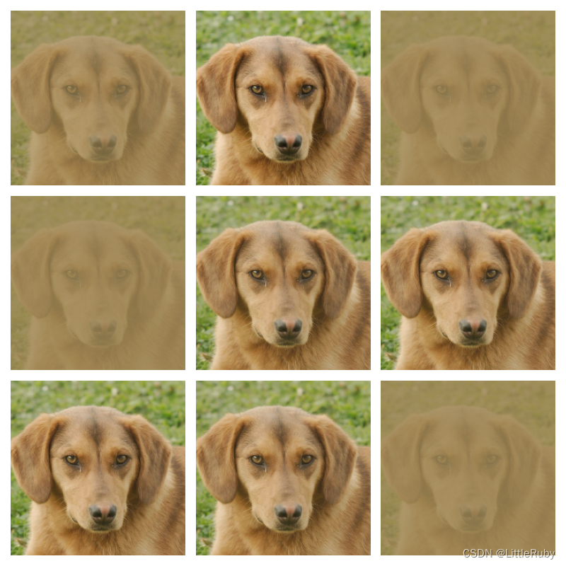

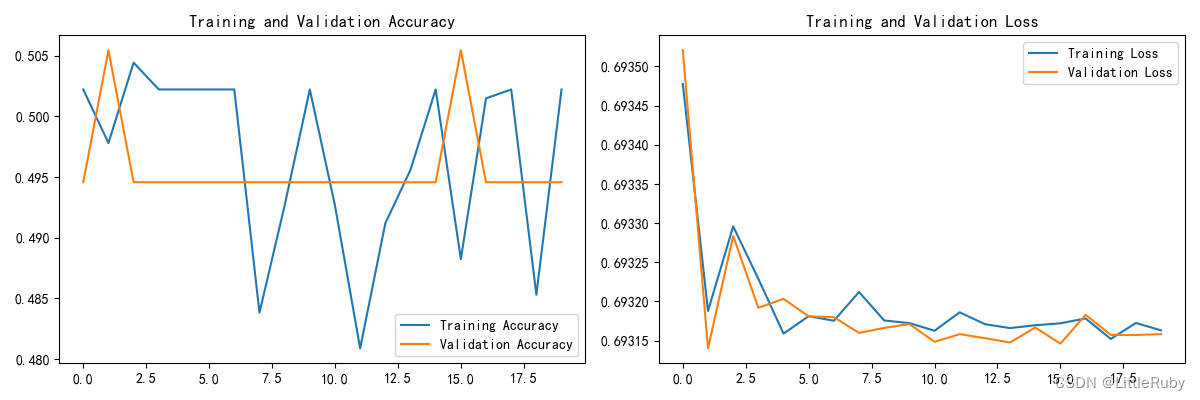
在這里插入圖片描述

效果也不是很理想，知道調用方法就行，針對不同案例實現圖像增強

1.3 圖像增強數據與原始數據合并作為新樣本

操作步驟如下：

讀取原始數據并圖像增強
保存增強效果圖
將原始數據與新生成的增強數據一起符號鏈接到新目錄

讀取原始數據并圖像增強，保存增強效果圖

from pathlib import Path
import cv2
import matplotlib.pyplot as plt
import warningswarnings.filterwarnings('ignore')  # 忽略一些warning內容，無需打印
def saveaugimg(imgfile,newdir,prefix="aug_"):# cv2保存中文路徑的圖像imgFile = imgfile  # 讀取文件的路徑img = cv2.imread(imgFile, flags=1)  # flags=1 讀取彩色圖像(BGR)img1 = cv2.flip(img, 2)  # 水平翻轉img2 = cv2.cvtColor(img1, cv2.COLOR_BGR2RGB)# plt.imshow(img2)# plt.show()saveFile = imgfile.replace(r"D:\DeepLearning\data\CatDog", newdir)  # 帶有中文的保存文件路徑newname=prefix+str(Path(imgfile).name)saveFile = Path(saveFile).parent / newnamePath(saveFile).parent.mkdir(parents=True, exist_ok=True)  # 創建新文件夾# cv2.imwrite(saveFile, img)  # imwrite 不支持中文路徑和文件名，讀取失敗，但不會報錯!img_write = cv2.imencode(".jpg", img1)[1].tofile(saveFile)dirs=r"D:\DeepLearning\data\CatDog"
newdir = r"D:\DeepLearning\data\CatDog_aug"
for p in Path(dirs).rglob("*"):if p.is_file():  # 如果是文件imgfile=str(p)saveaugimg(imgfile, newdir)

將原始數據與新生成的增強數據一起符號鏈接到新目錄

from pathlib import Path# 對目錄dirs做符號鏈接
def createslinkbatfile(dirs, slinkdirs, batfile="slink.bat"):print(f"為{dirs}創建符號鏈接目錄{slinkdirs}\n")# 創建符號鏈接目錄Path(slinkdirs).mkdir(parents=True, exist_ok=True)# 創建bat文件,為了解決bat腳本中文輸出亂碼問題，# 我們需要在bat腳本開頭添加chcp 65001來設置控制臺編碼格式為UTF-8。# 同時，我們還需要使用setlocal enabledelayedexpansion啟用延遲變量擴展with open(batfile, 'a', encoding='utf-8') as file:file.write("@echo off\nchcp 65001\nsetlocal enabledelayedexpansion " + '\n')# 遍歷目標目錄下的文件夾及文件，創建符號鏈接cmd命令for p in Path(dirs).rglob("*"):slink = Path(str(p).replace(str(dirs), str(slinkdirs)))  # 替換符號鏈接文件夾目錄if p.is_dir():  # 目錄符號鏈接command = f"mklink /d \"{slink}\" \"{str(p)}\""else:  # 文件符號鏈接command = f"mklink \"{slink}\" \"{str(p)}\""# 將符號鏈接cmd命令寫入bat文件with open(batfile, 'a', encoding='utf-8') as file:# 增加編碼encoding='utf-8'，解決中文亂碼問題解決方法file.write(command + '\n')print(command)# 對目錄dirs做符號鏈接,生成后右擊bat文件，選用管理員身份運行Path("slink.bat").unlink(missing_ok=False)# 刪除bat文件
dirs=r"D:\DeepLearning\data\CatDog"
newdirs = r"D:\DeepLearning\data\CatDog_aug"
slinkdirs = r"D:\DeepLearning\data\CatDog_all"
createslinkbatfile(dirs, slinkdirs)
createslinkbatfile(newdirs, slinkdirs)

部分bat內容同如下

@echo off
chcp 65001
setlocal enabledelayedexpansion 
mklink /d "D:\DeepLearning\data\CatDog_all\cat" "D:\DeepLearning\data\CatDog\cat"
mklink /d "D:\DeepLearning\data\CatDog_all\dog" "D:\DeepLearning\data\CatDog\dog"
mklink "D:\DeepLearning\data\CatDog_all\cat\flickr_cat_000002.jpg" "D:\DeepLearning\data\CatDog\cat\flickr_cat_000002.jpg"
mklink "D:\DeepLearning\data\CatDog_all\cat\flickr_cat_000003.jpg" "D:\DeepLearning\data\CatDog\cat\flickr_cat_000003.jpg"
mklink "D:\DeepLearning\data\CatDog_all\cat\flickr_cat_000004.jpg" "D:\DeepLearning\data\CatDog\cat\flickr_cat_000004.jpg"
mklink "D:\DeepLearning\data\CatDog_all\cat\flickr_cat_000005.jpg" "D:\DeepLearning\data\CatDog\cat\flickr_cat_000005.jpg"

tf.keras.preprocessing.image_dataset_from_directory（）傳入新的文件夾目錄

data_dir1 = r"D:\DeepLearning\data\CatDog_all"  # 將自定義數據增強后的數據保存后，與原始數據一起合并加入樣本中
data_dir = Path(data_dir1)

在這里插入圖片描述

總結

通過本次的學習，學習到了幾種圖像增強調用方式，原文中增強方式均為增強數據替代原始數據加入訓練集，本文加入將增強數據與原始數據一起合并作為樣本的方法，本文中的增強方式加入案例，效果并沒有很理想，跟數據集實際情況有關，可將本文提到的圖像增強方式運用到其他案例中。