導包

import numpy as np
from matplotlib import pyplot as plt
from sklearn.datasets import make_blobs

手寫數據劃分函數

x, y = make_blobs(n_samples = 300,n_features = 2,centers = 3,cluster_std = 1,center_box = (-10, 10),random_state = 666,return_centers = False
)

make_blobs：scikit-learn（sklearn）庫中的一個函數，用于生成聚類任務中的合成數據集。它可以生成具有指定特征數和聚類中心數的隨機數據集。

n_samples：生成的樣本總數，本例中為 300。
n_features：生成的每個樣本的特征數，本例中為 2。
centers：生成的簇的數量，本例中為 3。
cluster_std：每個簇中樣本的標準差，本例中為 1。
center_box：每個簇中心的邊界框（bounding box）范圍，本例中為 (-10, 10)。
random_state：隨機種子，用于控制數據的隨機性，本例中為 666。
return_centers：是否返回生成的簇中心點，默認為 False，在本例中不返回。

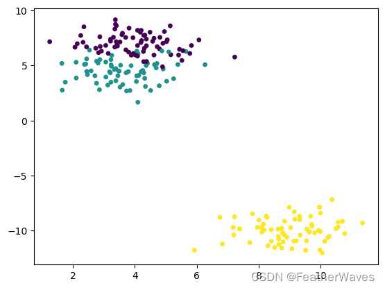
plt.scatter(x[:, 0], x[:, 1], c = y, s = 15)
plt.show()

x[:, 0]：表示取 x 數據集中所有樣本的第一個特征值。
x[:, 1]：表示取 x 數據集中所有樣本的第二個特征值。
c=y：表示使用標簽 y 對樣本點進行顏色編碼，即不同的標簽值將使用不同的顏色進行展示。
s=15：表示散點的大小為 15，即每個樣本點的顯示大小。

index = np.arange(20)
np.random.shuffle(index)
index

output: array([12, 15, 7, 11, 14, 16, 6, 5, 0, 1, 2, 19, 13, 4, 18, 9, 8,
10, 3, 17])

np.random.permutation(20)

output: array([ 6, 4, 11, 13, 18, 1, 8, 3, 10, 9, 7, 0, 15, 17, 19, 16, 5,
2, 14, 12])

np.random.seed(666)
shuffle = np.random.permutation(len(x))
shuffle

output:
array([235, 169, 17, 92, 234, 15, 0, 152, 176, 243, 98, 260, 96,
123, 266, 220, 109, 286, 185, 177, 160, 11, 50, 246, 258, 254,
34, 229, 154, 66, 285, 214, 237, 95, 7, 205, 262, 281, 110,
64, 111, 87, 263, 38, 153, 129, 273, 255, 208, 56, 162, 106,
277, 224, 178, 265, 108, 104, 101, 158, 248, 29, 181, 62, 14,
75, 118, 201, 41, 150, 131, 183, 288, 291, 76, 293, 267, 1,
165, 12, 278, 53, 209, 114, 71, 135, 184, 206, 244, 61, 211,
213, 128, 3, 143, 296, 227, 242, 94, 251, 284, 253, 89, 49,
159, 35, 268, 249, 197, 55, 167, 146, 23, 283, 187, 173, 124,
68, 250, 189, 186, 5, 221, 65, 40, 119, 74, 22, 19, 59,
188, 231, 44, 137, 31, 256, 43, 85, 149, 134, 218, 120, 81,
67, 239, 195, 207, 240, 182, 179, 90, 216, 180, 47, 299, 30,
163, 193, 48, 245, 138, 28, 257, 125, 170, 157, 259, 290, 200,
203, 215, 238, 194, 121, 298, 73, 97, 8, 130, 105, 190, 6,
36, 27, 32, 144, 4, 117, 115, 171, 136, 84, 10, 113, 233,
247, 72, 292, 198, 252, 82, 228, 37, 39, 33, 280, 272, 79,
116, 172, 202, 226, 271, 145, 13, 78, 196, 274, 26, 297, 191,
232, 52, 20, 230, 18, 58, 294, 140, 132, 287, 217, 25, 133,
83, 99, 93, 21, 241, 168, 147, 275, 212, 127, 54, 199, 282,
107, 151, 289, 88, 100, 264, 45, 77, 295, 9, 166, 57, 80,
155, 279, 86, 219, 2, 269, 126, 102, 142, 192, 161, 103, 42,
261, 16, 175, 122, 174, 164, 112, 148, 24, 139, 276, 141, 204,
210, 69, 46, 63, 225, 270, 156, 223, 60, 51, 222, 91, 70,
236])

np.random.seed(666)使得隨機數結果可復現

shuffle.shape

output: (300,)

train_size = 0.7
train_index = shuffle[:int(len(x) * train_size)]
test_index = shuffle[int(len(x) * train_size):]
train_index.shape, test_index.shape

output: ((210,), (90,))

x[train_index].shape, y[train_index].shape, x[test_index].shape, y[test_index].shape

output: ((210, 2), (210,), (90, 2), (90,))

def my_train_test_split(x, y, train_size = 0.7, random_state = None):if random_state:np.random.seed(random_state)shuffle = np.random.permutation(len(x))train_index = shuffle[:int(len(x) * train_size)]test_index = shuffle[int(len(x) * train_size):]return x[train_index], x[test_index], y[train_index], y[test_index]

x_train, x_test, y_train, y_test = my_train_test_split(x, y, train_size=0.7, random_state=233)
x_train.shape, x_test.shape, y_train.shape, y_test.shape

output: ((210, 2), (90, 2), (210,), (90,))

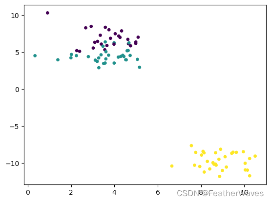
plt.scatter(x_train[:, 0], x_train[:, 1], c=y_train, s=15)  # y_train一樣的，顏色相同
plt.show()

plt.scatter(x_test[:, 0], x_test[:, 1], c=y_test, s=15)
plt.show()

使用sklearn內置的劃分數據函數

from sklearn.model_selection import train_test_split

x_train, x_test, y_train, y_test = train_test_split(x, y, train_size=0.7, random_state=233)
x_train.shape, x_test.shape, y_train.shape, y_test.shape

output: ((210, 2), (90, 2), (210,), (90,))

from collections import Counter
Counter(y_test)

output: Counter({2: 34, 0: 29, 1: 27})

x_train, x_test, y_train, y_test = train_test_split(x, y, train_size=0.7, random_state=666, stratify=y)

stratify=y： 使用標簽 y 進行分層采樣，確保訓練集和測試集中的類別分布相對一致。
這樣做的好處是，在訓練過程中，模型可以接觸到各個類別的樣本，從而更好地學習每個類別的特征和模式，提高模型的泛化能力。

Counter(y_test)

output: Counter({1: 30, 0: 30, 2: 30})

stratify=y理解舉例

x = np.random.randn(1000, 2)  # 1000個樣本，2個特征
y = np.concatenate([np.zeros(800), np.ones(200)])  # 800個負樣本，200個正樣本# 使用 stratify 進行分層采樣
x_train, x_test, y_train, y_test = train_test_split(x, y, train_size=0.7, random_state=42, stratify=y)# 打印訓練集中正負樣本的比例。通過使用 np.mean，我們可以方便地計算出比例或平均值，以了解數據集的分布情況或對模型性能進行評估。
print("訓練集中正樣本比例:", np.mean(y_train == 1))
print("訓練集中負樣本比例:", np.mean(y_train == 0))# 打印測試集中正負樣本的比例
print("測試集中正樣本比例:", np.mean(y_test == 1))
print("測試集中負樣本比例:", np.mean(y_test == 0))

output:
訓練集中正樣本比例: 0.2
訓練集中負樣本比例: 0.8
測試集中正樣本比例: 0.2
測試集中負樣本比例: 0.8