torch.clamp
主要用于對張量中的元素進行截斷(clamping),將其限制在一個指定的區間范圍內。
函數定義
torch.clamp(input, min=None, max=None) → Tensor參數說明
? ? input
? ? ? ? 類型:Tensor
? ? ? ? 需要進行截斷操作的輸入張量。
? ? min
? ? ? ? 類型:float 或 None(默認值)
? ? ? ? 指定張量中元素的最小值。小于 min 的元素會被截斷為 min 值。
? ? ? ? 如果設置為 None,則表示不限制最小值。
? ? max
? ? ? ? 類型:float 或 None(默認值)
? ? ? ? 指定張量中元素的最大值。大于 max 的元素會被截斷為 max 值。
? ? ? ? 如果設置為 None,則表示不限制最大值。
返回值
? ? 返回一個新的張量,其中元素已經被限制在 ([min, max]) 的范圍內。
? ? 原張量不會被修改(函數是非原地操作),除非使用 torch.clamp_ 以進行原地操作。
使用場景
torch.clamp 常見的應用場景包括:
- 避免數值溢出:限制張量中的數值在合理范圍內,防止出現過大或過小的值導致數值不穩定。
- 歸一化操作:將張量值限制在 [0, 1] 或 [-1, 1] 的范圍。
- 梯度截斷:在訓練神經網絡時避免梯度爆炸或梯度消失問題。
demo
僅設置最大值或最小值
x = torch.tensor([0.5, 2.0, -1.0, 3.0, -2.0])# 僅限制最大值為 1.0
result_max = torch.clamp(x, max=1.0)# 僅限制最小值為 0.0
result_min = torch.clamp(x, min=0.0)print(result_max)  # 輸出: tensor([0.5000, 1.0000, -1.0000, 1.0000, -2.0000])
print(result_min)  # 輸出: tensor([0.5000, 2.0000, 0.0000, 3.0000, 0.0000])
torch.nonzero
返回 input中非零元素的索引下標
無論輸入是幾維,輸出張量都是兩維,每行代表輸入張量中非零元素的索引位置(在所有維度上面的位置),行數表示非零元素的個數。
?
import torch
import torch.nn.functional as F
import mathX=torch.tensor([[0, 2, 0,  4],[5, 0, 7,  8]])
index = torch.nonzero(X)
# index = X.nonzero()
print(index)id_t = index.t_()
print(id_t)
tensor([[0, 1],
? ? ? ? [0, 3],
? ? ? ? [1, 0],
? ? ? ? [1, 2],
? ? ? ? [1, 3]])
tensor([[0, 0, 1, 1, 1],
? ? ? ? [1, 3, 0, 2, 3]])
?torch.sparse_coo_tensor
torch.sparse_coo_tensor(indices, values, size=None, *, dtype=None, device=None, requires_grad=False, check_invariants=None, is_coalesced=None)
創建一個Coordinate(COO) 格式的稀疏矩陣.
稀疏矩陣指矩陣中的大多數元素的值都為0,由于其中非常多的元素都是0,使用常規方法進行存儲非常的浪費空間,所以采用另外的方法存儲稀疏矩陣。

使用一個三元組來表示矩陣中的一個非0數,三元組分別表示元素(所在行,所在列,元素值),也就是上圖中每一個豎的三元組就是表示了一個非零數,其余值都為0,這樣就存儲了一個稀疏矩陣.構造這樣個矩陣需要知道所有非零數所在的行、所在的列、非零元素的值和矩陣的大小這四個值。
indices:此參數是指定非零元素所在的位置,也就是行和列,所以此參數應該是一個二維的數組,當然它可以是很多格式(ist, tuple, NumPy ndarray, scalar, and other types. )第一維指定了所有非零數所在的行數,第二維指定了所有非零元素所在的列數。例如indices=[[1, 4, 6], [3, 6, 7]]表示我們稀疏矩陣中(1, 3),(4, 6), (6, 7)幾個位置是非零的數所在的位置。
values:此參數指定了非零元素的值,所以此矩陣長度應該和上面的indices一樣長也可以是很多格式(list, tuple, NumPy ndarray, scalar, and other types.)。例如``values=[1, 4, 5]表示上面的三個位置非零數分別為1, 4, 5。
size:指定了稀疏矩陣的大小,例如size=[10, 10]表示矩陣大小為 10 × 10 10\times 10 10×10,此大小最小應該足以覆蓋上面非零元素所在的位置,如果不給定此值,那么默認是生成足以覆蓋所有非零值的最小矩陣大小。
dtype:指定返回tensor中數據的類型,如果不指定,那么采取values中數據的類型。
device:指定創建的tensor在cpu還是cuda上。
requires_grad:指定創建的tensor需不需要梯度信息,默認為False
import torchindices = torch.tensor([[4, 2, 1], [2, 0, 2]])
values = torch.tensor([3, 4, 5], dtype=torch.float32)
x = torch.sparse_coo_tensor(indices=indices, values=values, size=[5, 5])
print(x)
print('-----------------------------')
print(x.to_dense())
tensor(indices=tensor([[4, 2, 1],
? ? ? ? ? ? ? ? ? ? ? ?[2, 0, 2]]),
? ? ? ?values=tensor([3., 4., 5.]),
? ? ? ?size=(5, 5), nnz=3, layout=torch.sparse_coo)
-----------------------------
tensor([[0., 0., 0., 0., 0.],
? ? ? ? [0., 0., 5., 0., 0.],
? ? ? ? [4., 0., 0., 0., 0.],
? ? ? ? [0., 0., 0., 0., 0.],
? ? ? ? [0., 0., 3., 0., 0.]])
torch.max
import torch
import torch.nn.functional as F
import math# 創建一個二維張量
x = torch.tensor([[1, 3, 2], [4, 5, 6], [7, 8, 9]])# 返回最大值
value = torch.max(x)
print("value:", value)# 返回最大值及其索引
max_value, max_index = torch.max(x, 0)
print("Max value:", max_value)
print("Max index:", max_index)# 在第一個維度(行)上查找最大值,并保留形狀
max_value_row, max_index_row = torch.max(x, 0, keepdim=True)
print("dim=0 keeping shape: ", max_value_row)
print("dim=0 keeping shape: ", max_index_row)
value: tensor(9)
Max value: tensor([7, 8, 9])
Max index: tensor([2, 2, 2])
dim=0 keeping shape: ?tensor([[7, 8, 9]])
dim=0 keeping shape: ?tensor([[2, 2, 2]])
fastbev:
train
loss function?
F.binary_cross_entropy
F.binary_cross_entropy(
? ? input: Tensor, ?# 預測輸入
? ? target: Tensor, # 標簽
? ? weight: Optional[Tensor] = None, # 權重可選項
? ? size_average: Optional[bool] = None, ?# 可選項,快被棄用了
? ? reduce: Optional[bool] = None,
? ? reduction: str = "mean", ?# 默認均值或求和等形式
) -> Tensor:
?
?
input: 形狀為(N, *)的張量,表示模型的預測結果,取值范圍可以是任意實數。target: 形狀為(N, *)的張量,表示真實標簽,取值為 0 或 1。
import torch
import torch.nn.functional as F
import mathrow, col = 2, 3
x = torch.randn(row, col)predict = torch.sigmoid(x)index = torch.randint(col, size = (row,), dtype=torch.long)
y = torch.zeros(row, col)
y[range(y.shape[0]), index] = 1
print(range(y.shape[0]))loss1 = F.binary_cross_entropy(predict, y)
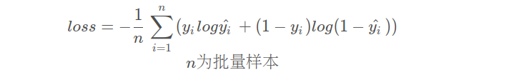
print("loss1 ",loss1)def binary_cross_entropy(predict, y):loss = -torch.sum(y * torch.log(predict) + (1 - y) * torch.log(1 - predict)) / torch.numel(y)return lossloss2 = binary_cross_entropy(predict, y)
print("loss2 ", loss2)range(0, 2)
loss1 ?tensor(1.1794)
loss2 ?tensor(1.1794)
F.binary_cross_entropy_with_logits
相比F.binary_cross_entropy函數,F.binary_cross_entropy_with_logits函數在內部使用了sigmoid函數.
F.binary_cross_entropy_with_logits = sigmoid +?F.binary_cross_entropy。
F.cross_entropy
多分類交叉熵損失函數
F.cross_entropy(input, target, weight=None, size_average=None, ignore_index=-100, reduce=None, reduction='mean')
參數說明:
? ? input:(N, C)形狀的張量,其中N為Batch_size,C為類別數。該參數對應于神經網絡最后一個全連接層輸出的未經Softmax處理的結果。
? ? target:一個大小為(N,)張量,其值是0 <= targets[i] <= C-1的元素,其中C是類別數。該參數包含一組給定的真實標簽(ground truth)。
? ? weight:采用類別平衡的加權方式計算損失值。可以傳入一個大小為(C,)張量,其中weight[j]是類別j的權重。默認為None。
? ? size_average:棄用,可以忽略。該參數已經被reduce參數取代了。
? ? ignore_index:指定被忽略的目標值的索引。如果目標值等于該索引,則不計算該樣本的損失。默認值為-100,即不忽略任何目標值。
? ? reduce:指定返回的損失值的方式。可以是“None”(不返回損失值)、“mean”(返回樣本損失值的平均值)和“sum”(返回樣本損失值的總和)。默認值為“mean”。
? ? reduction:與reduce參數等價。表示返回的損失值的方式。默認值為“mean”。

F.cross_entropy函數與nn.CrossEntropyLoss類是相似的,但前者更適合于控制更多的細節。
由于內部已經使用SoftMax函數處理,故兩者的輸入都不需要使用SoftMax處理。
import torch
import torch.nn.functional as F
import math# redictions:一個2維tensor,表示模型的預測結果。它的形狀是(2, 3),其中2是樣本數量,3是類別數量。每一行對應一個樣本的預測結果,每個元素表示該類別的概率。
# labels:一個1維tensor,表示樣本的真實標簽。它的形狀是(2,),其中2是樣本數量。
predictions = torch.tensor([[0.2, 0.3, 0.5], [0.8, 0.1, 0.1]])
labels = torch.tensor([2, 0])# 定義每個類別的權重
weights = torch.tensor([1.0, 2.0, 3.0])# 使用F.cross_entropy計算帶權重的交叉熵損失
loss = F.cross_entropy(predictions, labels, weight=weights)
print(loss) # tensor(0.8773)# 測試計算過程
pred = F.softmax(predictions, dim=1)
loss2 = -(weights[2] * math.log(pred[0, 2]) + weights[0]*math.log(pred[1, 0]))/4  # 4 = 1+3 對應權重之和
print(loss2) # 0.8773049571540321# 對于第一個樣本,它的預測結果為pred[0],真實標簽為2。根據交叉熵損失的定義,我們可以計算出它的損失為:
# -weights[2] * math.log(pred[0, 2])
# 對于第二個樣本,它的預測結果為pred[1],真實標簽為0。根據交叉熵損失的定義,我們可以計算出它的損失為:
# -weights[0] * math.log(pred[1, 0])
torch.nn.BCELoss
torch.nn.BCELoss(
? ? weight=None,?
? ? size_average=None,?
? ? reduce=None,?
? ? reduction='mean' # 默認計算的是批量樣本損失的平均值,還可以為'sum'或者'none'
)
?
torch.nn.BCEWithLogitsLoss
torch.nn.BCEWithLogitsLoss(
? ? weight=None,?
? ? size_average=None,?
? ? reduce=None,?
? ? reduction='mean', # 默認計算的是批量樣本損失的平均值,還可以為'sum'或者'none'
? ? pos_weight=None
)
?
import numpy as np
import torch
from torch import nn
import torch.nn.functional as Fy = torch.tensor([1, 0, 1], dtype=torch.float)
y_hat = torch.tensor([0.8, 0.2, 0.4], dtype=torch.float)bce_loss = nn.BCELoss()# nn.BCELoss()需要先對輸入數據進行sigmod
print("官方BCELoss = ", bce_loss(torch.sigmoid(y_hat), y))# nn.BCEWithLogitsLoss()不需要自己sigmod
bcelogits_loss = nn.BCEWithLogitsLoss()
print("官方BCEWithLogitsLoss = ", bcelogits_loss(y_hat, y))# 我們根據二分類交叉熵損失函數實現:
def loss(y_hat, y):y_hat = torch.sigmoid(y_hat)l = -(y * np.log(y_hat) + (1 - y) * np.log(1 - y_hat))l = sum(l) / len(l)return lprint('自己實現Loss = ', loss(y_hat, y))
# 可以看到結果值相同
官方BCELoss ? ? ? ? ? = ?tensor(0.5608)
官方BCEWithLogitsLoss = ?tensor(0.5608)
自己實現Loss ? ? ? ? ? = ?tensor(0.5608)
?
BCELoss與BCEWithLogitsLoss的關聯:BCEWithLogitsLoss = Sigmoid + BCELoss
import numpy as np
import torch
from torch import nn
import torch.nn.functional as Fy = torch.tensor([1, 0, 1], dtype=torch.float)
y_hat = torch.tensor([0.8, 0.2, 0.4], dtype=torch.float)bce_loss = nn.BCELoss()# nn.BCELoss()需要先對輸入數據進行sigmod
print("官方BCELoss = ", bce_loss(torch.sigmoid(y_hat), y))# nn.BCEWithLogitsLoss()不需要自己sigmod
bcelogits_loss = nn.BCEWithLogitsLoss()
print("官方BCEWithLogitsLoss = ", bcelogits_loss(y_hat, y))# 我們根據二分類交叉熵損失函數實現:
def loss(y_hat, y):y_hat = torch.sigmoid(y_hat)l = -(y * np.log(y_hat) + (1 - y) * np.log(1 - y_hat))l = sum(l) / len(l)return lprint('自己實現Loss = ', loss(y_hat, y))
# 可以看到結果值相同
官方BCELoss ? ? ? ? ? = ?tensor(0.5608)
官方BCEWithLogitsLoss = ?tensor(0.5608)
自己實現Loss ? ? ? ? ? = ?tensor(0.5608)
?
torch.nn.CrossEntropyLoss()
torch.nn.CrossEntropyLoss(
? ? weight=None,?
? ? size_average=None,?
? ? ignore_index=-100,?
? ? reduce=None,?
? ? reduction='mean',?
? ? label_smoothing=0.0 # 同樣,默認計算的是批量樣本損失的平均值,還可以為'sum'或者'none'
)
?
?
- 在關于二分類的問題中,輸入交叉熵公式的網絡預測值必須經過
Sigmoid進行映射 - 而在多分類問題中,需要將
Sigmoid替換成Softmax,這是兩者的一個重要區別 - CrossEntropyLoss =
softmax+log+nll_loss的集成
多分類交叉熵損失函數

 ?
?
cross_loss = nn.CrossEntropyLoss(reduction="none") # 設置為none,這里輸入每個樣本的loss值,不計算平均值
target = torch.tensor([0, 1, 2])predict = torch.tensor([[0.9, 0.2, 0.8],[0.5, 0.2, 0.4],[0.4, 0.2, 0.9]]) # 未經過softmax
print('官方實現CrossEntropyLoss: ', cross_loss(predict, target))# 自己實現方便理解版本的CrossEntropyLoss
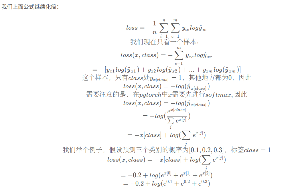
def cross_loss(predict, target, reduction=None):all_loss = []for index, value in enumerate(target):# 利用多分類簡化后的公式,對每一個樣本求loss值loss = -predict[index][value] + torch.log(sum(torch.exp(predict[index])))all_loss.append(loss)all_loss = torch.stack(all_loss)if reduction == 'none':return all_losselse:return torch.mean(all_loss)print('實現方便理解的CrossEntropyLoss: ', cross_loss(predict, target, reduction='none'))# 利用F.nll_loss實現的CrossEntropyLoss
def cross_loss2(predict, target, reduction=None):# Softmax的缺點:# 1、如果有得分值特別大的情況,會出現上溢情況;# 2、如果很小的負值很多,會出現下溢情況(超出精度范圍會向下取0),分母為0,導致計算錯誤。# 引入log_softmax可以解決上溢和下溢問題logsoftmax = F.log_softmax(predict)print('target = ', target)print('logsoftmax:\n', logsoftmax)# nll_loss不是將標簽值轉換為one-hot編碼,而是根據target的值,索引到對應元素,然后取相反數。loss = F.nll_loss(logsoftmax, target, reduction=reduction)return lossprint('F.nll_loss實現的CrossEntropyLoss: ', cross_loss2(predict, target, reduction='none'))
官方實現CrossEntropyLoss: ? ? ? ? ?tensor([0.8761, 1.2729, 0.7434])
實現方便理解的CrossEntropyLoss: ? ? tensor([0.8761, 1.2729, 0.7434])target = ?tensor([0, 1, 2])
logsoftmax:
tensor([[-0.8761, -1.5761, -0.9761],
? ? ? ? [-0.9729, -1.2729, -1.0729],
? ? ? ? [-1.2434, -1.4434, -0.7434]])
F.nll_loss實現的CrossEntropyLoss: ?tensor([0.8761, 1.2729, 0.7434])
??
)
:領導者/追隨者模式)

)


Java/python/JavaScript/C++/C語言/GO六種最佳實現)


