基于卷積神經網絡CNN，使用二維卷積Conv2D實現MNIST數字識別的四種方法

前言

系列專欄：機器學習：高級應用與實踐【項目實戰100+】【2024】??
在本專欄中不僅包含一些適合初學者的最新機器學習項目，每個項目都處理一組不同的問題，包括監督和無監督學習、分類、回歸和聚類，而且涉及創建深度學習模型、處理非結構化數據以及指導復雜的模型，如卷積神經網絡、門控循環單元、大型語言模型和強化學習模型

使用 MNIST 數據集進行手寫數字識別是一個借助神經網絡完成的重要項目。深度神經網絡是機器學習和人工智能的一個分支，這種網絡能夠從提供的無組織或無標記數據中進行無監督學習。

我們在此基礎上更進一步，我們的手寫數字識別系統不僅能檢測手寫數字的掃描圖像，還能借助集成的圖形用戶界面在屏幕上書寫數字進行識別。它主要檢測手寫數字的掃描圖像。

1. 相關庫和數據集
- 1.1 相關庫介紹
- 1.2 數據集介紹
2. 數據預處理
- 2.1 特征縮放
- 2.2 數據重塑
- 2.3 格式變換
3. 模型建立
- 3.1 數據準備
- 3.2 構建模型（4 種不同的模型結構）
- - 3.2.1 密集神經網絡
  - 3.2.2 二維卷積網絡（密集+最大池化）
  - 3.2.3 二維卷積網絡（密集+最大池化+Dropout）
  - 3.2.4 二維卷積網絡（密集+最大池化+Dropout+BN算法）
4. 模型評估
- 4.1 預測性能
- 4.2 比較結果
- 4.3 結果可視化

1. 相關庫和數據集

1.1 相關庫介紹

Python 庫使我們能夠非常輕松地處理數據并使用一行代碼執行典型和復雜的任務。

Numpy – 是一種開源的數值計算擴展，可用來存儲和處理大型矩陣，縮短大型計算的時間。
Matplotlib – 此庫用于繪制可視化效果，用于展現數據之間的相互關系。
TensorFlow? – 是一個基于數據流編程的符號數學系統，被廣泛應用于各類機器學習算法的編程實現。
Keras – 是一個由Python編寫的開源人工神經網絡庫，可以作為Tensorflow的高階應用程序接口，進行深度學習模型的設計、調試、評估、應用和可視化。

import numpy as np
import matplotlib.pyplot as pltfrom sklearn.model_selection import train_test_split
import tensorflow as tffrom tensorflow import keras
from tensorflow.keras import layers
from tensorflow.keras.datasets import mnist
from keras.utils import to_categorical

1.2 數據集介紹

MNIST 數據集是一組由中學生和美國人口普查局雇員手寫的 70,000 個小圖，由高中生和美國人口普查局的員工手寫而成。每個圖像都標有所代表的數字，人們對該數據集進行了大量研究，因此它經常被稱為機器學習的 “Hello World”。

(x_train, y_train), (x_test, y_test) = mnist.load_data()

print("Training Shape:", x_train.shape, y_train.shape)
print("----------------------------------------")
print("Testing Shape:", x_test.shape, y_test.shape)

Training Shape: (60000, 28, 28) (60000,)
----------------------------------------
Testing Shape: (10000, 28, 28) (10000,)

2. 數據預處理

2.1 特征縮放

①將像素值（0-255）歸一化為（0-1），以便更好地進行訓練

# Normalize pixel values (0-255) to (0-1) --> 0 for better training
x_train = x_train.astype('float32') / 255.0
x_test = x_test.astype('float32') / 255.0print("Min: %.3f, Max: %.3f" % (x_train.min(), x_train.max()))
print("Min: %.3f, Max: %.3f" % (x_test.min(), x_test.max()))

Min: 0.000, Max: 1.000
Min: 0.000, Max: 1.000

2.2 數據重塑

②重塑數據以便輸入神經網絡

# Reshape the data for input to the neural network (28x28 pixels)
x_train = x_train.reshape((x_train.shape[0], 28, 28, 1))
x_test = x_test.reshape((x_test.shape[0], 28, 28, 1))print("Training Shape:", x_train.shape)
print("----------------------------")
print("Testing Shape:", x_test.shape)

Training Shape: (60000, 28, 28, 1)
----------------------------
Testing Shape: (10000, 28, 28, 1)

2.3 格式變換

③將標簽從整數格式轉換為 one-hot 編碼向量

y_train = to_categorical(y_train, num_classes=10)
y_test = to_categorical(y_test, num_classes=10)print(y_train[0])
print(y_test[0])

[0. 0. 0. 0. 0. 1. 0. 0. 0. 0.]
[0. 0. 0. 0. 0. 0. 0. 1. 0. 0.]

3. 模型建立

3.1 數據準備

①將數據拆分為訓練數據、驗證數據和測試數據

x_train, x_val, y_train, y_val = train_test_split(x_train, y_train, test_size=0.20, random_state=1)

print("Training Shape:", x_train.shape, y_train.shape)
print("------------------------------------------")
print("validation Shape:", x_val.shape, y_val.shape)

Training Shape: (48000, 28, 28, 1) (48000, 10)
------------------------------------------
validation Shape: (12000, 28, 28, 1) (12000, 10)

3.2 構建模型（4 種不同的模型結構）

3.2.1 密集神經網絡

# 使用Sequential模型，并通過Input層指定輸入形狀
model_1 = keras.Sequential([layers.Input(shape=(28, 28, 1)),  # 這里的Input層定義了模型的輸入形狀layers.Flatten(),layers.Dense(512, activation='relu'),layers.Dense(256, activation='relu'),layers.Dense(10, activation='softmax')
])

# compile the model
model_1.compile(optimizer= 'adam',loss='categorical_crossentropy',metrics=['accuracy']
)

模型概要

model_1.summary()

Model: "sequential"
┏━━━━━━━━━━━━━━━━━━━━━━━━━━━━━━━━━━━━━━┳━━━━━━━━━━━━━━━━━━━━━━━━━━━━━┳━━━━━━━━━━━━━━━━━┓
┃ Layer (type)                         ┃ Output Shape                ┃         Param # ┃
┡━━━━━━━━━━━━━━━━━━━━━━━━━━━━━━━━━━━━━━╇━━━━━━━━━━━━━━━━━━━━━━━━━━━━━╇━━━━━━━━━━━━━━━━━┩
│ flatten (Flatten)                    │ (None, 784)                 │               0 │
├──────────────────────────────────────┼─────────────────────────────┼─────────────────┤
│ dense (Dense)                        │ (None, 512)                 │         401,920 │
├──────────────────────────────────────┼─────────────────────────────┼─────────────────┤
│ dense_1 (Dense)                      │ (None, 256)                 │         131,328 │
├──────────────────────────────────────┼─────────────────────────────┼─────────────────┤
│ dense_2 (Dense)                      │ (None, 10)                  │           2,570 │
└──────────────────────────────────────┴─────────────────────────────┴─────────────────┘Total params: 535,818 (2.04 MB)Trainable params: 535,818 (2.04 MB)Non-trainable params: 0 (0.00 B)

模型訓練

model_1.fit(x_train, y_train, validation_data=(x_val, y_val), epochs=10, batch_size=32)

Epoch 1/10
1500/1500 ━━━━━━━━━━━━━━━━━━━━ 6s 4ms/step - accuracy: 0.8948 - loss: 0.3426 - val_accuracy: 0.9642 - val_loss: 0.1150
Epoch 2/10
1500/1500 ━━━━━━━━━━━━━━━━━━━━ 4s 3ms/step - accuracy: 0.9745 - loss: 0.0825 - val_accuracy: 0.9719 - val_loss: 0.0933
Epoch 3/10
1500/1500 ━━━━━━━━━━━━━━━━━━━━ 5s 3ms/step - accuracy: 0.9829 - loss: 0.0534 - val_accuracy: 0.9727 - val_loss: 0.0980
Epoch 4/10
1500/1500 ━━━━━━━━━━━━━━━━━━━━ 4s 3ms/step - accuracy: 0.9865 - loss: 0.0380 - val_accuracy: 0.9709 - val_loss: 0.1073
Epoch 5/10
1500/1500 ━━━━━━━━━━━━━━━━━━━━ 4s 3ms/step - accuracy: 0.9892 - loss: 0.0302 - val_accuracy: 0.9778 - val_loss: 0.0905
Epoch 6/10
1500/1500 ━━━━━━━━━━━━━━━━━━━━ 4s 3ms/step - accuracy: 0.9927 - loss: 0.0225 - val_accuracy: 0.9760 - val_loss: 0.1015
Epoch 7/10
1500/1500 ━━━━━━━━━━━━━━━━━━━━ 4s 3ms/step - accuracy: 0.9936 - loss: 0.0186 - val_accuracy: 0.9775 - val_loss: 0.0990
Epoch 8/10
1500/1500 ━━━━━━━━━━━━━━━━━━━━ 5s 3ms/step - accuracy: 0.9933 - loss: 0.0196 - val_accuracy: 0.9778 - val_loss: 0.1068
Epoch 9/10
1500/1500 ━━━━━━━━━━━━━━━━━━━━ 4s 3ms/step - accuracy: 0.9939 - loss: 0.0182 - val_accuracy: 0.9772 - val_loss: 0.1158
Epoch 10/10
1500/1500 ━━━━━━━━━━━━━━━━━━━━ 4s 3ms/step - accuracy: 0.9938 - loss: 0.0182 - val_accuracy: 0.9770 - val_loss: 0.1083

模型評估

test_loss_1, test_accuracy_1 = model_1.evaluate(x_test, y_test)print("\nAccuracy =", test_accuracy_1, "\n-----------------------------", "\nLoss =", test_loss_1)

313/313 ━━━━━━━━━━━━━━━━━━━━ 2s 5ms/step - accuracy: 0.9749 - loss: 0.1182Accuracy = 0.978600025177002 
----------------------------- 
Loss = 0.09816069155931473

3.2.2 二維卷積網絡（密集+最大池化）

model_2 = keras.Sequential([layers.Input(shape=(28, 28, 1)),layers.Conv2D(32, (3,3), activation='relu'),layers.MaxPooling2D((2,2)),layers.Conv2D(64, (3,3), activation='relu'),layers.MaxPooling2D((2,2)),layers.Flatten(),layers.Dense(128, activation='relu'),layers.Dense(10, activation='softmax')
])

# compile the model
model_2.compile(optimizer= 'Adam',loss='categorical_crossentropy',metrics=['accuracy']
)

模型概要

model_2.summary()

Model: "sequential_1"
┏━━━━━━━━━━━━━━━━━━━━━━━━━━━━━━━━━━━━━━┳━━━━━━━━━━━━━━━━━━━━━━━━━━━━━┳━━━━━━━━━━━━━━━━━┓
┃ Layer (type)                         ┃ Output Shape                ┃         Param # ┃
┡━━━━━━━━━━━━━━━━━━━━━━━━━━━━━━━━━━━━━━╇━━━━━━━━━━━━━━━━━━━━━━━━━━━━━╇━━━━━━━━━━━━━━━━━┩
│ conv2d (Conv2D)                      │ (None, 26, 26, 32)          │             320 │
├──────────────────────────────────────┼─────────────────────────────┼─────────────────┤
│ max_pooling2d (MaxPooling2D)         │ (None, 13, 13, 32)          │               0 │
├──────────────────────────────────────┼─────────────────────────────┼─────────────────┤
│ conv2d_1 (Conv2D)                    │ (None, 11, 11, 64)          │          18,496 │
├──────────────────────────────────────┼─────────────────────────────┼─────────────────┤
│ max_pooling2d_1 (MaxPooling2D)       │ (None, 5, 5, 64)            │               0 │
├──────────────────────────────────────┼─────────────────────────────┼─────────────────┤
│ flatten_1 (Flatten)                  │ (None, 1600)                │               0 │
├──────────────────────────────────────┼─────────────────────────────┼─────────────────┤
│ dense_3 (Dense)                      │ (None, 128)                 │         204,928 │
├──────────────────────────────────────┼─────────────────────────────┼─────────────────┤
│ dense_4 (Dense)                      │ (None, 10)                  │           1,290 │
└──────────────────────────────────────┴─────────────────────────────┴─────────────────┘Total params: 225,034 (879.04 KB)Trainable params: 225,034 (879.04 KB)Non-trainable params: 0 (0.00 B)

模型訓練

model_2.fit(x_train, y_train, batch_size=32, validation_data=(x_val, y_val), epochs=10)

Epoch 1/10
1500/1500 ━━━━━━━━━━━━━━━━━━━━ 8s 5ms/step - accuracy: 0.9023 - loss: 0.3260 - val_accuracy: 0.9793 - val_loss: 0.0674
Epoch 2/10
1500/1500 ━━━━━━━━━━━━━━━━━━━━ 7s 4ms/step - accuracy: 0.9849 - loss: 0.0485 - val_accuracy: 0.9789 - val_loss: 0.0650
Epoch 3/10
1500/1500 ━━━━━━━━━━━━━━━━━━━━ 7s 4ms/step - accuracy: 0.9909 - loss: 0.0299 - val_accuracy: 0.9829 - val_loss: 0.0585
Epoch 4/10
1500/1500 ━━━━━━━━━━━━━━━━━━━━ 7s 4ms/step - accuracy: 0.9933 - loss: 0.0195 - val_accuracy: 0.9861 - val_loss: 0.0483
Epoch 5/10
1500/1500 ━━━━━━━━━━━━━━━━━━━━ 7s 4ms/step - accuracy: 0.9937 - loss: 0.0173 - val_accuracy: 0.9868 - val_loss: 0.0493
Epoch 6/10
1500/1500 ━━━━━━━━━━━━━━━━━━━━ 7s 4ms/step - accuracy: 0.9964 - loss: 0.0112 - val_accuracy: 0.9873 - val_loss: 0.0515
Epoch 7/10
1500/1500 ━━━━━━━━━━━━━━━━━━━━ 7s 4ms/step - accuracy: 0.9963 - loss: 0.0101 - val_accuracy: 0.9865 - val_loss: 0.0533
Epoch 8/10
1500/1500 ━━━━━━━━━━━━━━━━━━━━ 7s 4ms/step - accuracy: 0.9963 - loss: 0.0098 - val_accuracy: 0.9867 - val_loss: 0.0603
Epoch 9/10
1500/1500 ━━━━━━━━━━━━━━━━━━━━ 7s 4ms/step - accuracy: 0.9979 - loss: 0.0058 - val_accuracy: 0.9880 - val_loss: 0.0528
Epoch 10/10
1500/1500 ━━━━━━━━━━━━━━━━━━━━ 7s 4ms/step - accuracy: 0.9983 - loss: 0.0052 - val_accuracy: 0.9884 - val_loss: 0.0608

模型評估

test_loss_2, test_accuracy_2 = model_2.evaluate(x_test, y_test)print("\nAccuracy =", test_accuracy_2, "\n-----------------------------", "\nLoss =", test_loss_2)

313/313 ━━━━━━━━━━━━━━━━━━━━ 1s 2ms/step - accuracy: 0.9851 - loss: 0.0610Accuracy = 0.9889000058174133 
----------------------------- 
Loss = 0.046354446560144424

3.2.3 二維卷積網絡（密集+最大池化+Dropout）

model_3 = keras.Sequential([layers.Input(shape=(28, 28, 1)),layers.Conv2D(32, (3,3), activation='relu'),layers.MaxPooling2D((2,2)),layers.Conv2D(64, (3,3), activation='relu'),layers.MaxPooling2D((2,2)),layers.Conv2D(128, (3,3), activation='relu'),layers.Flatten(),layers.Dropout(0.5),layers.Dense(128, activation='relu'),layers.Dropout(0.5),layers.Dense(10, activation='softmax')
])

model_3.compile(optimizer='adam',loss='categorical_crossentropy',metrics=['accuracy']
)

模型概要

model_3.summary()

Model: "sequential_2"
┏━━━━━━━━━━━━━━━━━━━━━━━━━━━━━━━━━━━━━━┳━━━━━━━━━━━━━━━━━━━━━━━━━━━━━┳━━━━━━━━━━━━━━━━━┓
┃ Layer (type)                         ┃ Output Shape                ┃         Param # ┃
┡━━━━━━━━━━━━━━━━━━━━━━━━━━━━━━━━━━━━━━╇━━━━━━━━━━━━━━━━━━━━━━━━━━━━━╇━━━━━━━━━━━━━━━━━┩
│ conv2d_2 (Conv2D)                    │ (None, 26, 26, 32)          │             320 │
├──────────────────────────────────────┼─────────────────────────────┼─────────────────┤
│ max_pooling2d_2 (MaxPooling2D)       │ (None, 13, 13, 32)          │               0 │
├──────────────────────────────────────┼─────────────────────────────┼─────────────────┤
│ conv2d_3 (Conv2D)                    │ (None, 11, 11, 64)          │          18,496 │
├──────────────────────────────────────┼─────────────────────────────┼─────────────────┤
│ max_pooling2d_3 (MaxPooling2D)       │ (None, 5, 5, 64)            │               0 │
├──────────────────────────────────────┼─────────────────────────────┼─────────────────┤
│ conv2d_4 (Conv2D)                    │ (None, 3, 3, 128)           │          73,856 │
├──────────────────────────────────────┼─────────────────────────────┼─────────────────┤
│ flatten_2 (Flatten)                  │ (None, 1152)                │               0 │
├──────────────────────────────────────┼─────────────────────────────┼─────────────────┤
│ dropout (Dropout)                    │ (None, 1152)                │               0 │
├──────────────────────────────────────┼─────────────────────────────┼─────────────────┤
│ dense_5 (Dense)                      │ (None, 128)                 │         147,584 │
├──────────────────────────────────────┼─────────────────────────────┼─────────────────┤
│ dropout_1 (Dropout)                  │ (None, 128)                 │               0 │
├──────────────────────────────────────┼─────────────────────────────┼─────────────────┤
│ dense_6 (Dense)                      │ (None, 10)                  │           1,290 │
└──────────────────────────────────────┴─────────────────────────────┴─────────────────┘Total params: 241,546 (943.54 KB)Trainable params: 241,546 (943.54 KB)Non-trainable params: 0 (0.00 B)

模型訓練

model_3.fit(x_train, y_train, batch_size=32, validation_data=(x_val, y_val), epochs=10)

Epoch 1/10
1500/1500 ━━━━━━━━━━━━━━━━━━━━ 9s 5ms/step - accuracy: 0.8248 - loss: 0.5350 - val_accuracy: 0.9796 - val_loss: 0.0631
Epoch 2/10
1500/1500 ━━━━━━━━━━━━━━━━━━━━ 8s 5ms/step - accuracy: 0.9706 - loss: 0.0949 - val_accuracy: 0.9853 - val_loss: 0.0475
Epoch 3/10
1500/1500 ━━━━━━━━━━━━━━━━━━━━ 8s 5ms/step - accuracy: 0.9805 - loss: 0.0652 - val_accuracy: 0.9874 - val_loss: 0.0422
Epoch 4/10
1500/1500 ━━━━━━━━━━━━━━━━━━━━ 8s 5ms/step - accuracy: 0.9840 - loss: 0.0566 - val_accuracy: 0.9894 - val_loss: 0.0381
Epoch 5/10
1500/1500 ━━━━━━━━━━━━━━━━━━━━ 10s 5ms/step - accuracy: 0.9867 - loss: 0.0456 - val_accuracy: 0.9895 - val_loss: 0.0380
Epoch 6/10
1500/1500 ━━━━━━━━━━━━━━━━━━━━ 8s 5ms/step - accuracy: 0.9879 - loss: 0.0389 - val_accuracy: 0.9900 - val_loss: 0.0338
Epoch 7/10
1500/1500 ━━━━━━━━━━━━━━━━━━━━ 8s 5ms/step - accuracy: 0.9888 - loss: 0.0378 - val_accuracy: 0.9896 - val_loss: 0.0367
Epoch 8/10
1500/1500 ━━━━━━━━━━━━━━━━━━━━ 8s 5ms/step - accuracy: 0.9906 - loss: 0.0332 - val_accuracy: 0.9872 - val_loss: 0.0484
Epoch 9/10
1500/1500 ━━━━━━━━━━━━━━━━━━━━ 8s 5ms/step - accuracy: 0.9901 - loss: 0.0338 - val_accuracy: 0.9917 - val_loss: 0.0319
Epoch 10/10
1500/1500 ━━━━━━━━━━━━━━━━━━━━ 8s 5ms/step - accuracy: 0.9913 - loss: 0.0263 - val_accuracy: 0.9911 - val_loss: 0.0346

模型評估

test_loss_3, test_accuracy_3 = model_3.evaluate(x_test, y_test)print("\nAccuracy =", test_accuracy_3, "\n-----------------------------", "\nLoss =", test_loss_3)

313/313 ━━━━━━━━━━━━━━━━━━━━ 1s 2ms/step - accuracy: 0.9883 - loss: 0.0389Accuracy = 0.991100013256073 
----------------------------- 
Loss = 0.030680162832140923

3.2.4 二維卷積網絡（密集+最大池化+Dropout+BN算法）

model_4 = keras.Sequential([layers.Input(shape=(28, 28, 1)),layers.Conv2D(32, (3,3), activation='relu'),layers.BatchNormalization(),layers.MaxPooling2D((2,2)),layers.Conv2D(64, (3,3), activation='relu'),layers.BatchNormalization(),layers.MaxPooling2D((2,2)),layers.Conv2D(128, (3,3), activation='relu'),layers.Flatten(),layers.Dropout(0.2),             # using 20% dropout instead of 50%layers.Dense(128, activation='relu'),layers.Dropout(0.2),layers.Dense(10, activation='softmax'),
])

model_4.compile(optimizer='adam',loss='categorical_crossentropy',metrics=['accuracy']
)

模型概要

model_4.summary()

Model: "sequential_3"
┏━━━━━━━━━━━━━━━━━━━━━━━━━━━━━━━━━━━━━━┳━━━━━━━━━━━━━━━━━━━━━━━━━━━━━┳━━━━━━━━━━━━━━━━━┓
┃ Layer (type)                         ┃ Output Shape                ┃         Param # ┃
┡━━━━━━━━━━━━━━━━━━━━━━━━━━━━━━━━━━━━━━╇━━━━━━━━━━━━━━━━━━━━━━━━━━━━━╇━━━━━━━━━━━━━━━━━┩
│ conv2d_5 (Conv2D)                    │ (None, 26, 26, 32)          │             320 │
├──────────────────────────────────────┼─────────────────────────────┼─────────────────┤
│ batch_normalization                  │ (None, 26, 26, 32)          │             128 │
│ (BatchNormalization)                 │                             │                 │
├──────────────────────────────────────┼─────────────────────────────┼─────────────────┤
│ max_pooling2d_4 (MaxPooling2D)       │ (None, 13, 13, 32)          │               0 │
├──────────────────────────────────────┼─────────────────────────────┼─────────────────┤
│ conv2d_6 (Conv2D)                    │ (None, 11, 11, 64)          │          18,496 │
├──────────────────────────────────────┼─────────────────────────────┼─────────────────┤
│ batch_normalization_1                │ (None, 11, 11, 64)          │             256 │
│ (BatchNormalization)                 │                             │                 │
├──────────────────────────────────────┼─────────────────────────────┼─────────────────┤
│ max_pooling2d_5 (MaxPooling2D)       │ (None, 5, 5, 64)            │               0 │
├──────────────────────────────────────┼─────────────────────────────┼─────────────────┤
│ conv2d_7 (Conv2D)                    │ (None, 3, 3, 128)           │          73,856 │
├──────────────────────────────────────┼─────────────────────────────┼─────────────────┤
│ flatten_3 (Flatten)                  │ (None, 1152)                │               0 │
├──────────────────────────────────────┼─────────────────────────────┼─────────────────┤
│ dropout_2 (Dropout)                  │ (None, 1152)                │               0 │
├──────────────────────────────────────┼─────────────────────────────┼─────────────────┤
│ dense_7 (Dense)                      │ (None, 128)                 │         147,584 │
├──────────────────────────────────────┼─────────────────────────────┼─────────────────┤
│ dropout_3 (Dropout)                  │ (None, 128)                 │               0 │
├──────────────────────────────────────┼─────────────────────────────┼─────────────────┤
│ dense_8 (Dense)                      │ (None, 10)                  │           1,290 │
└──────────────────────────────────────┴─────────────────────────────┴─────────────────┘Total params: 241,930 (945.04 KB)Trainable params: 241,738 (944.29 KB)Non-trainable params: 192 (768.00 B)

模型訓練

model_4.fit(x_train, y_train, batch_size=64, validation_data=(x_val, y_val), epochs=6)

Epoch 1/6
750/750 ━━━━━━━━━━━━━━━━━━━━ 12s 14ms/step - accuracy: 0.9043 - loss: 0.3018 - val_accuracy: 0.9855 - val_loss: 0.0485
Epoch 2/6
750/750 ━━━━━━━━━━━━━━━━━━━━ 10s 13ms/step - accuracy: 0.9841 - loss: 0.0517 - val_accuracy: 0.9862 - val_loss: 0.0458
Epoch 3/6
750/750 ━━━━━━━━━━━━━━━━━━━━ 10s 13ms/step - accuracy: 0.9882 - loss: 0.0379 - val_accuracy: 0.9881 - val_loss: 0.0442
Epoch 4/6
750/750 ━━━━━━━━━━━━━━━━━━━━ 10s 13ms/step - accuracy: 0.9906 - loss: 0.0286 - val_accuracy: 0.9873 - val_loss: 0.0452
Epoch 5/6
750/750 ━━━━━━━━━━━━━━━━━━━━ 10s 13ms/step - accuracy: 0.9923 - loss: 0.0252 - val_accuracy: 0.9845 - val_loss: 0.0545
Epoch 6/6
750/750 ━━━━━━━━━━━━━━━━━━━━ 10s 13ms/step - accuracy: 0.9923 - loss: 0.0236 - val_accuracy: 0.9871 - val_loss: 0.0486

模型評估

test_loss_4, test_accuracy_4 = model_4.evaluate(x_test, y_test)print("\nAccuracy =", test_accuracy_4, "\n-----------------------------", "\nLoss =", test_loss_4)

313/313 ━━━━━━━━━━━━━━━━━━━━ 1s 2ms/step - accuracy: 0.9856 - loss: 0.0679Accuracy = 0.9901000261306763 
----------------------------- 
Loss = 0.04728936031460762

4. 模型評估

4.1 預測性能

①構建模型性能預測函數

def predict(model, image):reshaped_image = image.reshape((1, 28, 28, 1))prediction = model.predict(reshaped_image)predicted_class = np.argmax(prediction)return predicted_class

predict_image_class = predict(model_1, x_test[0])
print("Predicted Class Label: ", predict_image_class)
print("Actual Class Label of the same image:",(np.argmax(y_test[0])))

1/1 ━━━━━━━━━━━━━━━━━━━━ 0s 38ms/step
Predicted Class Label:  7
Actual Class Label of the same image: 7

4.2 比較結果

def compare_models(models, x_test, y_test):accuracies = []model_names = []for model in models:_, accuracy = model.evaluate(x_test, y_test)accuracies.append(accuracy)best_model_index = np.argmax(accuracies)best_model = models[best_model_index]best_accuracy = accuracies[best_model_index]model_names = [f"Model {i+1}" for i in range(len(models))]plt.plot(model_names, accuracies, marker='o')plt.xlabel('Models')plt.ylabel('Accuracy')plt.title('Comparison of Model Accuracies')plt.xticks(rotation=45)plt.show()print("Comparison Results:")for i in range(len(models)):print(f"Model {i+1} - Accuracy: { accuracies[i]:.4f}")print(f"Best Model : Model {best_model_index+1}")print(f"Best Accuracy: {best_accuracy:.4f}")return best_model

models = [model_1, model_2, model_3, model_4]
best_model = compare_models(models, x_test, y_test)

313/313 ━━━━━━━━━━━━━━━━━━━━ 1s 2ms/step - accuracy: 0.9749 - loss: 0.1182
313/313 ━━━━━━━━━━━━━━━━━━━━ 1s 2ms/step - accuracy: 0.9851 - loss: 0.0610
313/313 ━━━━━━━━━━━━━━━━━━━━ 1s 2ms/step - accuracy: 0.9883 - loss: 0.0389
313/313 ━━━━━━━━━━━━━━━━━━━━ 1s 2ms/step - accuracy: 0.9856 - loss: 0.0679

4.3 結果可視化

評估結果可視化

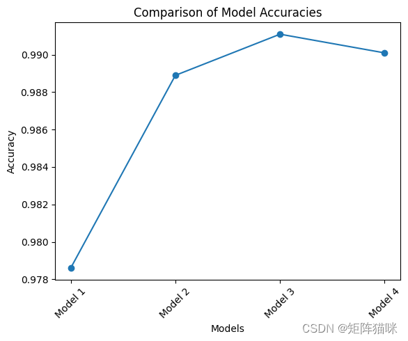
Comparison Results:
Model 1 - Accuracy: 0.9786
Model 2 - Accuracy: 0.9889
Model 3 - Accuracy: 0.9911
Model 4 - Accuracy: 0.9901
Best Model : Model 3
Best Accuracy: 0.9911