優化理論

本章節介紹深度學習中的高級優化技術，包括學習率衰減、梯度裁剪和批量歸一化。這些技術能夠顯著提升模型的訓練效果和穩定性。

學習率衰減（Learning Rate Decay）

數學原理與可視化

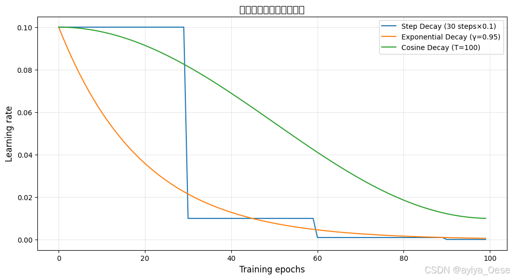
學習率衰減策略的數學表達：

1. 步進式衰減：
   $${\alpha }_t={\alpha }_0\times {\gamma }^{?t/s?}$$
   其中$s$為衰減周期，$\gamma$為衰減因子

2. 指數衰減：
   $${\alpha }_t={\alpha }_0\times e^{?\gamma t}$$

3. 余弦衰減：
   $${\alpha }_t={\alpha }_{\text{min}}+\frac{1}{2}({\alpha }_0?{\alpha }_{\text{min}})(1+\cos (\frac{t\pi }{T}))$$

import matplotlib.pyplot as plt# 衰減策略可視化
epochs = 100
initial_lr = 0.1# 計算各策略學習率
step_lrs = [initial_lr * (0.1 ** (i//30)) for i in range(epochs)]
expo_lrs = [initial_lr * (0.95 ** i) for i in range(epochs)]
cosine_lrs = [0.01 + 0.5*(0.1-0.01)*(1 + np.cos(np.pi*i/epochs)) for i in range(epochs)]# 繪制對比圖
plt.figure(figsize=(12,6))
plt.plot(step_lrs, label='Step Decay (每30步×0.1)')
plt.plot(expo_lrs, label='Exponential Decay (γ=0.95)')
plt.plot(cosine_lrs, label='Cosine Decay (T=100)')
plt.title("不同學習率衰減策略對比", fontsize=14)
plt.xlabel("訓練周期", fontsize=12)
plt.ylabel("學習率", fontsize=12)
plt.legend()
plt.grid(True, alpha=0.3)

最佳實踐

# 組合使用多種調度器
optimizer = torch.optim.SGD(model.parameters(), lr=0.1)# 前50步使用余弦衰減
scheduler1 = CosineAnnealingLR(optimizer, T_max=50)
# 之后使用步進衰減
scheduler2 = StepLR(optimizer, step_size=10, gamma=0.5)for epoch in range(100):train(...)if epoch < 50:scheduler1.step()else:scheduler2.step()

---

梯度裁剪（Gradient Clipping）

數學原理

梯度裁剪通過限制梯度范數防止參數更新過大：
$$\text{if?}\Vert g\Vert >c:g\leftarrow \frac{c}{\Vert g\Vert }g$$
其中$c$為裁剪閾值，$\Vert g\Vert$為梯度范數

梯度動態可視化

import torch
import torch.nn as nn
import torch.optim as optim
import matplotlib.pyplot as plt# 定義一個簡單的模型
class SimpleModel(nn.Module):def __init__(self):super(SimpleModel, self).__init__()self.fc = nn.Linear(10, 1)def forward(self, x):return self.fc(x)# 初始化模型、優化器和損失函數
model = SimpleModel()
optimizer = optim.SGD(model.parameters(), lr=0.01)
criterion = nn.MSELoss()grad_norms = []
clipped_grad_norms = []for _ in range(1000):# 生成隨機輸入和目標inputs = torch.randn(32, 10)targets = torch.randn(32, 1)# 前向傳播outputs = model(inputs)loss = criterion(outputs, targets)# 反向傳播optimizer.zero_grad()loss.backward()# 記錄裁剪前梯度grad_norms.append(torch.norm(torch.cat([p.grad.view(-1) for p in model.parameters()])))# 執行裁剪torch.nn.utils.clip_grad_norm_(model.parameters(), max_norm=1.0)# 記錄裁剪后梯度clipped_grad_norms.append(torch.norm(torch.cat([p.grad.view(-1) for p in model.parameters()])))# 更新參數optimizer.step()# 繪制梯度變化
plt.figure(figsize=(12, 6))
plt.plot(grad_norms, alpha=0.6, label='Original Gradient Norm')
plt.plot(clipped_grad_norms, alpha=0.6, label='Clipped Gradient Norm')
plt.axhline(1.0, color='r', linestyle='--', label='Clipping Threshold')
plt.yscale('log')
plt.title("Gradient Clipping Effect Monitoring", fontsize=14)
plt.xlabel("Training Steps", fontsize=12)
plt.ylabel("Gradient L2 Norm (log scale)", fontsize=12)
plt.legend()
plt.grid(True, alpha=0.3)
plt.show()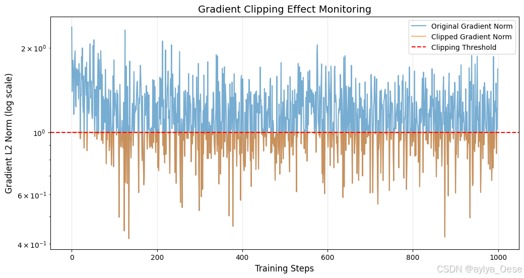

實踐技巧

1. RNN中推薦值：LSTM/GRU 中 max_norm 取 1.0 或 2.0
2. 結合學習率：較高學習率需配合較小裁剪閾值
3. 監控策略：定期輸出梯度統計量

print(f"梯度均值: {grad.mean().item():.3e} ± {grad.std().item():.3e}")

---

批量歸一化（Batch Normalization）

數學推導

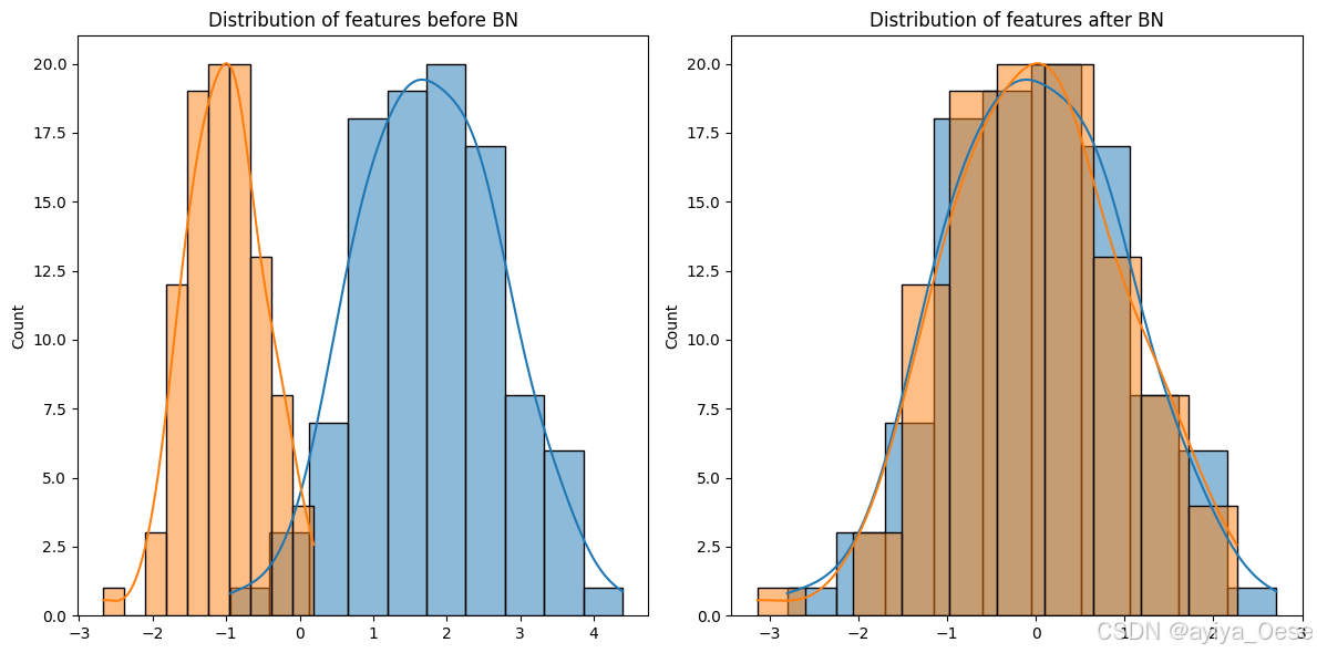
對于輸入批次 B = { x 1 , . . . , x m } B = \{x_1,...,x_m\} B={x1?,...,xm?}：

1. 計算統計量：
   $$\begin{gathered} {\mu }_B=\frac{1}{m}\sum _{i=1}^m{x}_i \\ {\sigma }_B^2=\frac{1}{m}\sum _{i=1}^m(x_i?{\mu }_B{)}^2 \end{gathered}$$
2. 標準化：
   $${\hat{x}}_i=\frac{x_i?{\mu }_B}{\sqrt{{\sigma }_B^2+?}}$$
3. 仿射變換：
   $$y_i=\gamma {\hat{x}}_i+\beta$$

訓練/評估模式對比

import torch.nn as nn
import torch
# 創建BN層
bn = nn.BatchNorm1d(64)# 訓練模式
bn.train()
for _ in range(100):x = torch.randn(32, 64)  # 批大小32y = bn(x)
print("訓練模式統計:", bn.running_mean[:5].detach().numpy())  # 顯示部分通道# 評估模式
bn.eval()
with torch.no_grad():x = torch.randn(32, 64)y = bn(x)
print("評估模式統計:", bn.running_mean[:5].detach().numpy())

可視化BN效果

# 生成模擬數據
data = torch.cat([torch.normal(2.0, 1.0, (100, 1)),torch.normal(-1.0, 0.5, (100, 1))
], dim=1)# 應用BN
bn = nn.BatchNorm1d(2)
output = bn(data)# 繪制分布對比
plt.figure(figsize=(12,6))
plt.subplot(1,2,1)
sns.histplot(data[:,0], kde=True, label='原始特征1')
sns.histplot(data[:,1], kde=True, label='原始特征2')
plt.title("Distribution of features before BN")plt.subplot(1,2,2)
sns.histplot(output[:,0], kde=True, label='BN后特征1')
sns.histplot(output[:,1], kde=True, label='BN后特征2') 
plt.title("Distribution of features after BN")plt.tight_layout()

---

技術組合應用案例

圖像分類任務

# 自定義CNN模型
class CustomCNN(nn.Module):def __init__(self):super().__init__()# 卷積層 使用BNself.conv_layers = nn.Sequential(nn.Conv2d(3, 64, 3),nn.BatchNorm2d(64),nn.ReLU(),nn.MaxPool2d(2),nn.Conv2d(64, 128, 3),nn.BatchNorm2d(128),nn.ReLU(),nn.MaxPool2d(2),)# 全連接層self.fc = nn.Linear(128*5*5, 10)def forward(self, x):x = self.conv_layers(x)return self.fc(x.view(x.size(0), -1))# 初始化模型、優化器和調度器
model = CustomCNN()
optimizer = torch.optim.SGD(model.parameters(), lr=0.1, momentum=0.9, weight_decay=1e-4)
scheduler = CosineAnnealingLR(optimizer, T_max=200)# 帶梯度裁剪的訓練循環
max_grad_norm = 5.0  # 裁剪閾值
for epoch in range(200):model.train()  # 模型進入訓練模式for inputs, targets in train_loader:  # 訓練數據加載器outputs = model(inputs)  # 前向傳播loss = F.cross_entropy(outputs, targets)  # 計算損失optimizer.zero_grad()  # 梯度清零loss.backward()  # 反向傳播# 梯度裁剪torch.nn.utils.clip_grad_norm_(model.parameters(), max_grad_norm)optimizer.step()  # 參數更新scheduler.step()  # 學習率更新

---

關鍵技術總結

技術	主要作用	典型應用場景	注意事項
學習率衰減	精細收斂	深層網絡訓練	配合warmup效果更佳
梯度裁剪	穩定訓練	RNN、Transformer	閾值需隨batch size調整
批量歸一化	加速收斂	CNN、全連接網絡	小batch效果差

組合策略建議

1. CNN架構：BN + 動量SGD + 余弦衰減
2. RNN架構：梯度裁剪 + Adam + 步進衰減
3. Transformer：預熱 + 梯度裁剪 + AdamW

# Transformer優化示例
optimizer = torch.optim.AdamW(model.parameters(), lr=3e-4, betas=(0.9, 0.98))
scheduler = torch.optim.lr_scheduler.LambdaLR(optimizer,lr_lambda=lambda step: min(step**-0.5, step*(4000**-1.5))  # 預熱
)