通透！手把教你如何從頭構建一個機器學習模型

1.業務理解

2.數據收集和準備

數據采集

探索性數據分析 (EDA) 和數據清理

特征選擇

3.建立機器學習模型

選擇正確的模型

分割數據

訓練模型

模型評估

4.模型優化

5.部署模型

今天我將帶領大家一步步的來構建一個機器學習模型。

我們將按照以下步驟開發客戶流失預測分類模型。

文末福利：拉到最后

包含：Java、云原生、GO語音、嵌入式、Linux、物聯網、AI人工智能、python、C/C++/C#、軟件測試、網絡安全、Web前端、網頁、大數據、Android大模型多線程、JVM、Spring、MySQL、Redis、Dubbo、中間件…等最全廠牌最新視頻教程+源碼+軟件包+面試必考題和答案詳解。

1.業務理解

在開發任何機器學習模型之前，我們必須了解為什么要開發該模型。

這里，我們以客戶流失預測為例。

在這種情況下，企業需要避免公司進一步流失，并希望對流失概率高的客戶采取行動。有了上述業務需求，所以需要開發一個客戶流失預測模型。

2.數據收集和準備

數據采集

數據是任何機器學習項目的核心。沒有數據，我們就無法訓練機器學習模型。

在現實情況下，干凈的數據并不容易獲得。通常，我們需要通過應用程序、調查和許多其他來源收集數據，然后將其存儲在數據存儲中。

在我們的案例中，我們將使用來自 Kaggle 的電信客戶流失數據。它是有關電信行業客戶歷史的開源分類數據，帶有流失標簽。

https://www.kaggle.com/datasets/blastchar/telco-customer-churn

探索性數據分析 (EDA) 和數據清理

首先，我們加載數據集。

import?pandas?as?pddf?=?pd.read_csv('WA_Fn-UseC_-Telco-Customer-Churn.csv')
df.head()

接下來，我們將探索數據以了解我們的數據集。

以下是我們將為 EDA 流程執行的一些操作。

檢查特征和匯總統計數據。
檢查特征中是否存在缺失值。
分析標簽的分布（流失）。
為數值特征繪制直方圖，為分類特征繪制條形圖。
為數值特征繪制相關熱圖。
使用箱線圖識別分布和潛在異常值。

首先，我們將檢查特征和匯總統計數據。

df.info()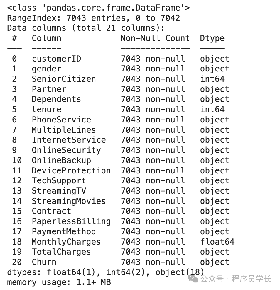

df.describe()df.describe(exclude?=?'number')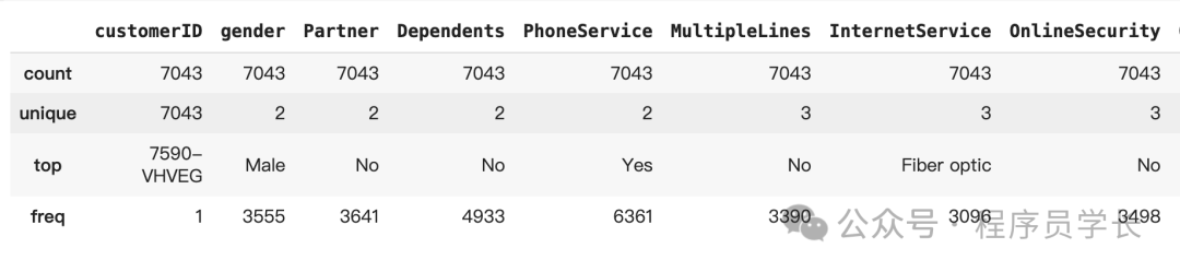

讓我們檢查一下缺失的數據。

df.isnull().sum()

可以看到，數據集不包含缺失數據，因此我們不需要執行任何缺失數據處理活動。

然后，我們將檢查目標變量以查看是否存在不平衡情況。

df['Churn'].value_counts()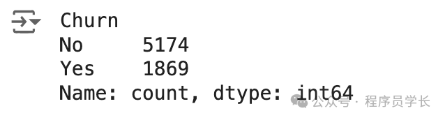

存在輕微的不平衡，因為與無客戶流失的情況相比，只有接近 25% 的客戶流失發生。

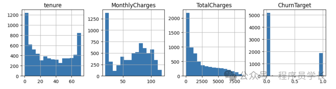
讓我們再看看其他特征的分布情況，從數字特征開始。

import?numpy?as?np
df['TotalCharges']?=?df['TotalCharges'].replace('',?np.nan)
df['TotalCharges']?=?pd.to_numeric(df['TotalCharges'],?errors='coerce').fillna(0)

df['SeniorCitizen']?=?df['SeniorCitizen'].astype('str')

df['ChurnTarget']?=?df['Churn'].apply(lambda?x:?1?if?x=='Yes'?else?0)

num_features?=?df.select_dtypes('number').columns
df[num_features].hist(bins=15,?figsize=(15,?6),?layout=(2,?5))

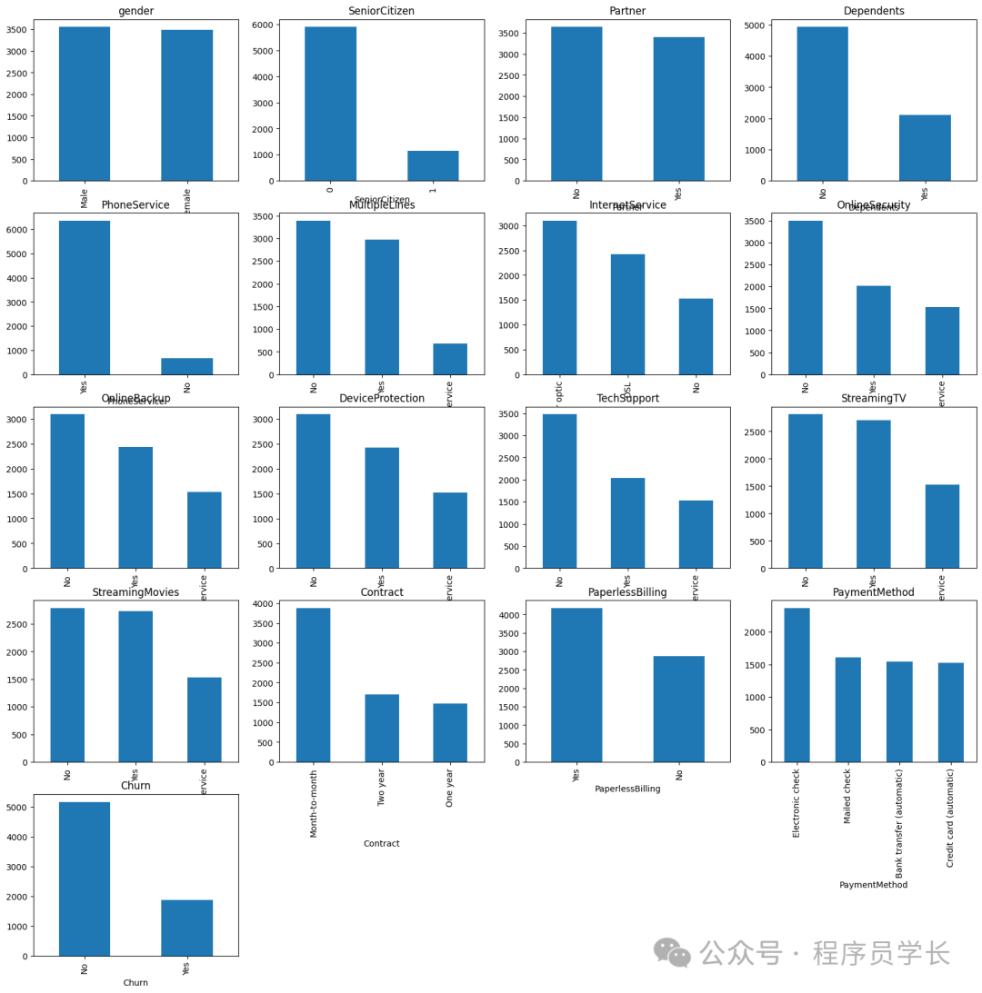
我們還將提供除 customerID 之外的分類特征繪圖。

import?matplotlib.pyplot?as?plt
#?Plot?distribution?of?categorical?features
cat_features?=?df.drop('customerID',?axis?=1).select_dtypes(include='object').columns

plt.figure(figsize=(20,?20))
for?i,?col?in?enumerate(cat_features,?1):
????plt.subplot(5,?4,?i)
????df[col].value_counts().plot(kind='bar')
????plt.title(col)

然后我們將通過以下代碼看到數值特征之間的相關性。

import?seaborn?as?sns#?Plot?correlations?between?numerical?features
plt.figure(figsize=(10,?8))
sns.heatmap(df[num_features].corr())
plt.title('Correlation?Heatmap')

最后，我們將使用基于四分位距（IQR）的箱線圖檢查數值異常值。

#?Plot?box?plots?to?identify?outliers
plt.figure(figsize=(20,?15))
for?i,?col?in?enumerate(num_features,?1):plt.subplot(4,?4,?i)sns.boxplot(y=df[col])plt.title(col)

從上面的分析中，我們可以看出，我們不應該解決缺失數據或異常值的問題。

下一步是對我們的機器學習模型進行特征選擇，因為我們只想要那些影響預測且在業務中可行的特征。

特征選擇

特征選擇的方法有很多種，通常結合業務知識和技術應用來完成。

但是，本教程將僅使用我們之前做過的相關性分析來進行特征選擇。

首先，讓我們根據相關性分析選擇數值特征。

target?=?'ChurnTarget'
num_features?=?df.select_dtypes(include=[np.number]).columns.drop(target)#?Calculate?correlations
correlations?=?df[num_features].corrwith(df[target])#?Set?a?threshold?for?feature?selection
threshold?=?0.3
selected_num_features?=?correlations[abs(correlations)?>?threshold].index.tolist()
selected_cat_features=cat_features[:-1]selected_features?=?[]
selected_features.extend(selected_num_features)
selected_features.extend(selected_cat_features)
selected_features

你可以稍后嘗試調整閾值，看看特征選擇是否會影響模型的性能。

3.建立機器學習模型

選擇正確的模型

選擇合適的機器學習模型需要考慮很多因素，但始終取決于業務需求。

以下幾點需要記住：

用例問題。它是監督式的還是無監督式的？是分類式的還是回歸式的？用例問題將決定可以使用哪種模型。
數據特征。它是表格數據、文本還是圖像？數據集大小是大還是小？根據數據集的不同，我們選擇的模型可能會有所不同。
模型的解釋難度如何？平衡可解釋性和性能對于業務至關重要。

經驗法則是，在開始復雜模型之前，最好先以較簡單的模型作為基準。

對于本教程，我們從邏輯回歸開始進行模型開發。

分割數據

下一步是將數據拆分為訓練、測試和驗證集。

from?sklearn.model_selection?import?train_test_splittarget?=?'ChurnTarget'?X?=?df[selected_features]
y?=?df[target]cat_features?=?X.select_dtypes(include=['object']).columns.tolist()
num_features?=?X.select_dtypes(include=['number']).columns.tolist()#Splitting?data?into?Train,?Validation,?and?Test?Set
X_train_val,?X_test,?y_train_val,?y_test?=?train_test_split(X,?y,?test_size=0.2,?random_state=42,?stratify=y)X_train,?X_val,?y_train,?y_val?=?train_test_split(X_train_val,?y_train_val,?test_size=0.25,?random_state=42,?stratify=y_train_val)

在上面的代碼中，我們將數據分成 60% 的訓練數據集和 20% 的測試和驗證集。

一旦我們有了數據集，我們就可以訓練模型。

訓練模型

如上所述，我們將使用訓練數據訓練 Logistic 回歸模型。

from?sklearn.compose?import?ColumnTransformer
from?sklearn.pipeline?import?Pipeline
from?sklearn.preprocessing?import?OneHotEncoder
from?sklearn.linear_model?import?LogisticRegressionpreprocessor?=?ColumnTransformer(transformers=[('num',?'passthrough',?num_features),('cat',?OneHotEncoder(),?cat_features)])pipeline?=?Pipeline(steps=[('preprocessor',?preprocessor),('classifier',?LogisticRegression(max_iter=1000))
])#?Train?the?logistic?regression?model
pipeline.fit(X_train,?y_train)

模型評估

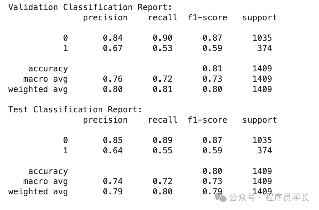
以下代碼顯示了所有基本分類指標。

from?sklearn.metrics?import?classification_report#?Evaluate?on?the?validation?set
y_val_pred?=?pipeline.predict(X_val)
print("Validation?Classification?Report:\n",?classification_report(y_val,?y_val_pred))#?Evaluate?on?the?test?set
y_test_pred?=?pipeline.predict(X_test)
print("Test?Classification?Report:\n",?classification_report(y_test,?y_test_pred))

從驗證和測試數據中我們可以看出，流失率(1) 的召回率并不是最好的。這就是為什么我們可以優化模型以獲得最佳結果。

4.模型優化

優化模型的一種方法是通過超參數優化，它會測試這些模型超參數的所有組合，以根據指標找到最佳組合。

每個模型都有一組超參數，我們可以在訓練之前設置它們。

from?sklearn.model_selection?import?GridSearchCV
#?Define?the?logistic?regression?model?within?a?pipeline
pipeline?=?Pipeline(steps=[('preprocessor',?preprocessor),('classifier',?LogisticRegression(max_iter=1000))
])#?Define?the?hyperparameters?for?GridSearchCV
param_grid?=?{'classifier__C':?[0.1,?1,?10,?100],'classifier__solver':?['lbfgs',?'liblinear']
}#?Perform?Grid?Search?with?cross-validation
grid_search?=?GridSearchCV(pipeline,?param_grid,?cv=5,?scoring='recall')
grid_search.fit(X_train,?y_train)#?Best?hyperparameters
print("Best?Hyperparameters:",?grid_search.best_params_)#?Evaluate?on?the?validation?set
y_val_pred?=?grid_search.predict(X_val)
print("Validation?Classification?Report:\n",?classification_report(y_val,?y_val_pred))#?Evaluate?on?the?test?set
y_test_pred?=?grid_search.predict(X_test)
print("Test?Classification?Report:\n",?classification_report(y_test,?y_test_pred))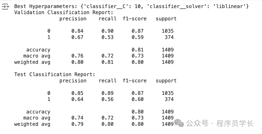

5.部署模型

我們已經構建了機器學習模型。有了模型之后，下一步就是將其部署到生產中。讓我們使用一個簡單的 API 來模擬它。

首先，讓我們再次開發我們的模型并將其保存為 joblib 對象。

import?joblibbest_params?=?{'classifier__C':?10,?'classifier__solver':?'liblinear'}
logreg_model?=?LogisticRegression(C=best_params['classifier__C'],?solver=best_params['classifier__solver'],?max_iter=1000)preprocessor?=?ColumnTransformer(transformers=[('num',?'passthrough',?num_features),('cat',?OneHotEncoder(),?cat_features)])pipeline?=?Pipeline(steps=[('preprocessor',?preprocessor),('classifier',?logreg_model)
])pipeline.fit(X_train,?y_train)#?Save?the?model
joblib.dump(pipeline,?'logreg_model.joblib')

一旦模型對象準備就緒，我們將創建一個名為 app.py 的 Python 腳本，并將以下代碼放入腳本中。

from?fastapi?import?FastAPI
from?pydantic?import?BaseModel
import?joblib
import?numpy?as?np#?Load?the?logistic?regression?model?pipeline
model?=?joblib.load('logreg_model.joblib')#?Define?the?input?data?for?model
class?CustomerData(BaseModel):tenure:?intInternetService:?strOnlineSecurity:?strTechSupport:?strContract:?strPaymentMethod:?str#?Create?FastAPI?app
app?=?FastAPI()#?Define?prediction?endpoint
@app.post("/predict")
def?predict(data:?CustomerData):input_data?=?{'tenure':?[data.tenure],'InternetService':?[data.InternetService],'OnlineSecurity':?[data.OnlineSecurity],'TechSupport':?[data.TechSupport],'Contract':?[data.Contract],'PaymentMethod':?[data.PaymentMethod]}import?pandas?as?pdinput_df?=?pd.DataFrame(input_data)#?Make?a?predictionprediction?=?model.predict(input_df)#?Return?the?predictionreturn?{"prediction":?int(prediction[0])}if?__name__?==?"__main__":import?uvicornuvicorn.run(app,?host="0.0.0.0",?port=8000)

在命令提示符或終端中，運行以下代碼。

uvicorn?app:app?--reload

有了上面的代碼，我們已經有一個用于接受數據和創建預測的 API。

讓我們在新終端中使用以下代碼嘗試一下。

curl?-X?POST?"http://127.0.0.1:8000/predict"?-H?"Content-Type:?application/json"?-d?"{\"tenure\":?72,?\"InternetService\":?\"Fiber?optic\",?\"OnlineSecurity\":?\"Yes\",?\"TechSupport\":?\"Yes\",?\"Contract\":?\"Two?year\",?\"PaymentMethod\":?\"Credit?card?(automatic)\"}"

如你所見，API 結果是一個預測值為 0（Not-Churn）的字典。你可以進一步調整代碼以獲得所需的結果。