歡迎大家關注全網生信學習者系列:
- WX公zhong號:生信學習者
- Xiao hong書:生信學習者
- 知hu:生信學習者
- CDSN:生信學習者2
介紹
計算配對微生物在組間的相關關系波動情況進而評估不同分組的微生物狀態。secom_linear 函數可以評估不同分組(例如,健康組與疾病組)中微生物分類群之間的線性相關性,幫助研究者理解不同分類群如何相互作用以及它們在不同狀態下的相互關系。通過分析不同分組間微生物相關性的波動情況,secom_linear 函數能夠揭示微生物群落結構的動態變化,這對于理解微生物群落對環境變化的響應至關重要。
在不同分組之間,微生物分類群的相互關系表現出顯著的波動性。這種波動性反映了微生物群落結構在不同環境或條件下的動態變化,是評估微生物群落穩定性和功能多樣性的關鍵指標。通過定量分析這些波動,研究者可以深入理解微生物群落如何響應外部擾動,以及它們在不同生態位中的作用和相互依賴性。
加載R包
library(readr)
library(openxlsx)
library(tidyverse)
library(igraph)
library(ggraph)
library(tidygraph)
library(ggpubr)
library(microbiome)
library(ANCOMBC)
導入數據
大家通過以下鏈接下載數據:
- 百度網盤鏈接:https://pan.baidu.com/s/1fz5tWy4mpJ7nd6C260abtg
- 提取碼: 請關注WX公zhong號_生信學習者_后臺發送 復現gmsb 獲取提取碼
otu_table <- read_tsv("./data/GMSB-data/otu-table.tsv", show_col_types = FALSE)tax <- read_tsv("./data/GMSB-data/taxonomy.tsv", show_col_types = FALSE)meta_data <- read_csv("./data/GMSB-data/df_v1.csv", show_col_types = FALSE)
數據預處理
- 提取差異物種豐度表
- 合并分組變量和差異物種豐度表
Primary group: 按照頻率分組
-
G1: # receptive anal intercourse = 0
-
G2: # receptive anal intercourse = 1
-
G3: # receptive anal intercourse = 2 - 5
-
G4: # receptive anal intercourse = 6 +
# OTU table
otu_id <- otu_table$`#OTU ID`
otu_table <- data.frame(otu_table[, -1], check.names = FALSE, row.names = otu_id)# Taxonomy table
otu_id <- tax$`Feature ID`
tax <- data.frame(tax[, - c(1, 3)], row.names = otu_id)
tax <- tax %>% separate(col = Taxon, into = c("Kingdom", "Phylum", "Class", "Order", "Family", "Genus", "Species"),sep = ";") %>%rowwise() %>%dplyr::mutate_all(function(x) strsplit(x, "__")[[1]][2]) %>%mutate(Species = ifelse(!is.na(Species) & !is.na(Genus),paste(ifelse(strsplit(Genus, "")[[1]][1] == "[",strsplit(Genus, "")[[1]][2],strsplit(Genus, "")[[1]][1]), Species, sep = "."),NA)) %>%ungroup()
tax <- as.matrix(tax)
rownames(tax) <- otu_id
tax[tax == ""] <- NA# Meta data
meta_data$status <- factor(meta_data$status, levels = c("nc", "sc"))
meta_data$time2aids <- factor(meta_data$time2aids,levels = c("never", "> 10 yrs","5 - 10 yrs", "< 5 yrs"))# Phyloseq object
OTU <- otu_table(otu_table, taxa_are_rows = TRUE)
META <- sample_data(meta_data)
sample_names(META) <- meta_data$sampleid
TAX <- tax_table(tax)
otu_data <- phyloseq(OTU, TAX, META)
species_data <- aggregate_taxa(otu_data, "Species")tse <- mia::makeTreeSummarizedExperimentFromPhyloseq(otu_data)
tse <- tse[, tse$group1 != "missing"]
tse1 <- tse[, tse$group1 == "g1"]
tse2 <- tse[, tse$group1 == "g2"]
tse3 <- tse[, tse$group1 == "g3"]
tse4 <- tse[, tse$group1 == "g4"]tse4key_species <- c("A.muciniphila", "B.caccae", "B.fragilis", "B.uniformis","Bacteroides spp.", "Butyricimonas spp.", "Dehalobacterium spp.", "Methanobrevibacter spp.", "Odoribacter spp.")
class: TreeSummarizedExperiment
dim: 6111 35
metadata(0):
assays(1): counts
rownames(6111): 000e1601e0051888d502cd6a535ecdda 0011d81f43ec49d21f2ab956ab12de2f ...fff3a05f150a52a2b6c238d2926a660d fffc6ea80dc6bb8cafacbab2d3b157b3
rowData names(7): Kingdom Phylum ... Genus Species
colnames(35): F-195 F-133 ... F-368 F-377
colData names(45): sampleid subjid ... hbv hcv
reducedDimNames(0):
mainExpName: NULL
altExpNames(0):
rowLinks: NULL
rowTree: NULL
colLinks: NULL
colTree: NULL
函數
-
get_upper_tri:獲取上三角矩陣結果 -
data_preprocess:獲取相關性畫圖矩陣
get_upper_tri <- function(cormat){cormat[lower.tri(cormat)] <- NAdiag(cormat) <- NAreturn(cormat)
}data_preprocess <- function(res, type = "linear", level = "Species", tax) {if (type == "linear") {df_corr <- res$corr_fl} else {df_corr <- res$dcorr_fl}if (level == "Species") {tax_name <- colnames(df_corr)tax_name <- sapply(tax_name, function(x) {name <- ifelse(grepl("Genus:", x), paste(strsplit(x, ":")[[1]][2], "spp."),ifelse(grepl("Species:", x), strsplit(x, ":")[[1]][2], x))return(name)})colnames(df_corr) <- tax_namerownames(df_corr) <- tax_namedf_corr <- df_corr[tax, tax]} else {tax_name <- colnames(df_corr)tax_name <- sapply(tax_name, function(x) strsplit(x, ":")[[1]][2])colnames(df_corr) <- tax_namerownames(df_corr) <- tax_namedf_corr <- df_corr[tax, tax]}tax_name <- sort(colnames(df_corr))df_corr <- df_corr[tax_name, tax_name]df_clean <- data.frame(get_upper_tri(df_corr)) %>%rownames_to_column("var1") %>%pivot_longer(cols = -var1, names_to = "var2", values_to = "value") # Correct for namesdf_name <- data.frame(var1 = unique(df_clean$var1),var2 = unique(df_clean$var2))for (i in seq_len(nrow(df_name))) {df_clean$var2[df_clean$var2 == df_name$var2[i]] = df_name$var1[i]}df_clean <- df_clean %>%filter(!is.na(value)) %>%mutate(value = round(value, 2))return(df_clean)
}
Linear correlations
secom_linear 函數是 ANCOMBC 包中的一個函數,用于在微生物組數據中進行線性相關性的稀疏估計。該函數支持三種相關性系數的計算:皮爾遜(Pearson)、斯皮爾曼(Spearman)和肯德爾(Kendall’s tau)相關系數。以下是 secom_linear 函數的主要參數和它們的作用:
- data: 包含微生物組數據的列表。
- assay_name: 指定數據集中的哪個檢測類型(如“counts”)。
- tax_level: 指定使用的分類水平,例如“Phylum”(門)。
- pseudo: 偽計數,用于穩定稀疏矩陣的計算。
- prv_cut: 用于過濾掉低豐度的物種的閾值。
- lib_cut: 用于過濾掉低測序深度的樣本的閾值。
- corr_cut: 用于過濾掉低相關性的閾值。
- wins_quant: 用于確定窗口大小的分位數。
- method: 指定計算哪種相關性系數,可以是“pearson”、“spearman”。
- soft: 是否使用軟閾值。
- thresh_len: 硬閾值的長度。
- n_cv: 交叉驗證的迭代次數。
- thresh_hard: 硬閾值,用于確定最終的相關性矩陣。
- max_p: 最大 p 值,用于多重測試校正。
- n_cl: 聚類的數量。
函數會返回兩個主要的結果對象:corr_th 和 corr_fl,分別代表閾值相關性矩陣和完整相關性矩陣。這些矩陣提供了不同物種或分類水平之間的線性相關性估計。
Run SECOM
secom_linear 函數1)首先通過設置不同的閾值來過濾數據,2)然后使用指定的方法計算相關性系數,3)并通過交叉驗證等技術來確定最終的相關性矩陣。這個過程涉及到數據的預處理、相關性計算和結果的后處理,以確保相關性估計的準確性和稀疏性。
set.seed(123)res_linear1 <- ANCOMBC::secom_linear(data = list(tse1), assay_name = "counts",tax_level = "Species", pseudo = 0, prv_cut = 0.1, lib_cut = 1000, corr_cut = 0.5,wins_quant = c(0.05, 0.95), method = "pearson",soft = FALSE, thresh_len = 20, n_cv = 10,thresh_hard = 0.3, max_p = 0.005, n_cl = 2)names(res_linear1)res_linear2 <- ANCOMBC::secom_linear(data = list(tse2), assay_name = "counts",tax_level = "Species", pseudo = 0,prv_cut = 0.1, lib_cut = 1000, corr_cut = 0.5,wins_quant = c(0.05, 0.95), method = "pearson", soft = FALSE, thresh_len = 20, n_cv = 10, thresh_hard = 0.3, max_p = 0.005, n_cl = 2)res_linear3 <- ANCOMBC::secom_linear(data = list(tse3), assay_name = "counts",tax_level = "Species", pseudo = 0, prv_cut = 0.1, lib_cut = 1000, corr_cut = 0.5,wins_quant = c(0.05, 0.95), method = "pearson",soft = FALSE, thresh_len = 20, n_cv = 10, thresh_hard = 0.3, max_p = 0.005, n_cl = 2)res_linear4 <- ANCOMBC::secom_linear(data = list(tse4), assay_name = "counts",tax_level = "Species", pseudo = 0, prv_cut = 0.1, lib_cut = 1000, corr_cut = 0.5,wins_quant = c(0.05, 0.95), method = "pearson",soft = FALSE, thresh_len = 20, n_cv = 10, thresh_hard = 0.3, max_p = 0.005, n_cl = 2)species1 <- rownames(res_linear1$corr_fl)
species1 <- species1[grepl("Species:", species1)|grepl("Genus:", species1)]
species2 <- rownames(res_linear2$corr_fl)
species2 <- species2[grepl("Species:", species2)|grepl("Genus:", species2)]
species3 <- rownames(res_linear3$corr_fl)
species3 <- species3[grepl("Species:", species3)|grepl("Genus:", species3)]
species4 <- rownames(res_linear4$corr_fl)
species4 <- species4[grepl("Species:", species4)|grepl("Genus:", species4)]
common_species <- Reduce(intersect, list(species1, species2, species3, species4))
common_species <- sapply(common_species, function(x) ifelse(grepl("Genus:", x), paste(strsplit(x, ":")[[1]][2], "spp."),strsplit(x, ":")[[1]][2]))
[1] "s_diff_hat" "y_hat" "cv_error" "thresh_grid" "thresh_opt" "mat_cooccur" "corr" "corr_p" [9] "corr_th" "corr_fl"
結果:四個分組的線性相關的共有物種,查看微生物兩兩之間的相關系數
Visualization
可視化同一組微生物兩兩之間的相關系數在不同組的變化狀態
df_corr1 <- data_preprocess(res_linear1, type = "linear", level = "Species", tax = key_species) %>%dplyr::mutate(group = "G1")
df_corr2 <- data_preprocess(res_linear2, type = "linear", level = "Species", tax = key_species) %>%dplyr::mutate(group = "G2")
df_corr3 <- data_preprocess(res_linear3, type = "linear", level = "Species", tax = key_species) %>%dplyr::mutate(group = "G3")
df_corr4 <- data_preprocess(res_linear4, type = "linear", level = "Species", tax = key_species) %>%dplyr::mutate(group = "G4")df_corr <- do.call('rbind', list(df_corr1, df_corr2, df_corr3, df_corr4)) %>%unite("pair", var1:var2, sep = " vs. ")value_check <- df_corr %>%dplyr::group_by(pair) %>%dplyr::summarise(empty_idx = ifelse(all(value == 0), TRUE, FALSE))non_empty_pair <- value_check %>%filter(empty_idx == FALSE) %>%.$pair
df_fig <- df_corr %>%dplyr::filter(pair %in% non_empty_pair)fig_species_linear <- df_fig %>%ggline(x = "group", y = "value",color = "steelblue", facet.by = "pair",xlab = "Correlation coefficient", ylab = "", title = "Pearson Correlation") +scale_y_continuous(breaks = seq(0, 0.8, 0.2), limits = c(0, 0.9)) +geom_text(aes(label = round(value, 2)), vjust = -0.5) +theme(plot.title = element_text(hjust = 0.5))fig_species_linear
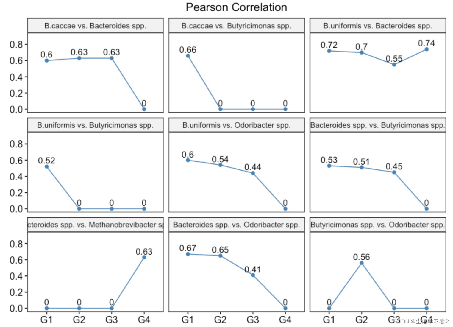
結果:同一微生物對兩兩之間的相關關系在不同分組不同,這可能表明不同狀態下,微生物之間的相關關系不一樣或意味著不同的微生物模式。
Nonlinear correlations
secom_linear 函數是 ANCOMBC 包中的一個函數,用于在微生物組數據中進行線性相關性的稀疏估計。該函數支持三種相關性系數的計算:皮爾遜(Pearson)、斯皮爾曼(Spearman)和肯德爾(Kendall’s tau)相關系數。以下是 secom_linear 函數的主要參數和它們的作用:
- data: 包含微生物組數據的列表。
- assay_name: 指定數據集中的哪個檢測類型(如“counts”)。
- tax_level: 指定使用的分類水平,例如“Phylum”(門)。
- pseudo: 偽計數,用于穩定稀疏矩陣的計算。
- prv_cut: 用于過濾掉低豐度的物種的閾值。
- lib_cut: 用于過濾掉低測序深度的樣本的閾值。
- corr_cut: 用于過濾掉低相關性的閾值。
- wins_quant: 用于確定窗口大小的分位數。
- method: 指定計算哪種相關性系數,可以是“pearson”、“spearman”。
- soft: 是否使用軟閾值。
- thresh_len: 硬閾值的長度。
- n_cv: 交叉驗證的迭代次數。
- thresh_hard: 硬閾值,用于確定最終的相關性矩陣。
- max_p: 最大 p 值,用于多重測試校正。
- n_cl: 聚類的數量。
函數會返回兩個主要的結果對象:corr_th 和 corr_fl,分別代表閾值相關性矩陣和完整相關性矩陣。這些矩陣提供了不同物種或分類水平之間的線性相關性估計。
Run SECOM
secom_linear 函數1)首先通過設置不同的閾值來過濾數據,2)然后使用指定的方法計算相關性系數,3)并通過交叉驗證等技術來確定最終的相關性矩陣。這個過程涉及到數據的預處理、相關性計算和結果的后處理,以確保相關性估計的準確性和稀疏性。
set.seed(123)res_dist1 <- ANCOMBC::secom_dist(data = list(tse1), assay_name = "counts",tax_level = "Species", pseudo = 0, prv_cut = 0.1, lib_cut = 1000, corr_cut = 0.5,wins_quant = c(0.05, 0.95),R = 1000, thresh_hard = 0.3, max_p = 0.005, n_cl = 2)res_dist2 <- ANCOMBC::secom_dist(data = list(tse2), assay_name = "counts",tax_level = "Species", pseudo = 0,prv_cut = 0.1, lib_cut = 1000, corr_cut = 0.5,wins_quant = c(0.05, 0.95),R = 1000, thresh_hard = 0.3, max_p = 0.005, n_cl = 2)res_dist3 <- ANCOMBC::secom_dist(data = list(tse3), assay_name = "counts",tax_level = "Species", pseudo = 0, prv_cut = 0.1, lib_cut = 1000, corr_cut = 0.5,wins_quant = c(0.05, 0.95),R = 1000, thresh_hard = 0.3, max_p = 0.005, n_cl = 2)res_dist4 <- ANCOMBC::secom_dist(data = list(tse4), assay_name = "counts",tax_level = "Species", pseudo = 0,prv_cut = 0.1, lib_cut = 1000, corr_cut = 0.5,wins_quant = c(0.05, 0.95),R = 1000, thresh_hard = 0.3, max_p = 0.005, n_cl = 2)species1 <- rownames(res_dist1$corr_fl)
species1 <- species1[grepl("Species:", species1)|grepl("Genus:", species1)]
species2 <- rownames(res_dist2$corr_fl)
species2 <- species2[grepl("Species:", species2)|grepl("Genus:", species2)]
species3 <- rownames(res_dist3$corr_fl)
species3 <- species3[grepl("Species:", species3)|grepl("Genus:", species3)]
species4 <- rownames(res_dist4$corr_fl)
species4 <- species4[grepl("Species:", species4)|grepl("Genus:", species4)]
common_species <- Reduce(intersect, list(species1, species2, species3, species4))
common_species <- sapply(common_species, function(x) ifelse(grepl("Genus:", x), paste(strsplit(x, ":")[[1]][2], "spp."),strsplit(x, ":")[[1]][2]))
結果:四個分組的線性相關的共有物種,查看微生物兩兩之間的相關系數
Visualization
可視化同一組微生物兩兩之間的相關系數在不同組的變化狀態
df_corr1 <- data_preprocess(res_dist1, type = "dist", level = "Species", tax = key_species) %>%dplyr::mutate(group = "G1")
df_corr2 <- data_preprocess(res_dist2, type = "dist", level = "Species", tax = key_species) %>%dplyr::mutate(group = "G2")
df_corr3 <- data_preprocess(res_dist3, type = "dist", level = "Species", tax = key_species) %>%dplyr::mutate(group = "G3")
df_corr4 <- data_preprocess(res_dist4, type = "dist", level = "Species", tax = key_species) %>%dplyr::mutate(group = "G4")df_corr <- do.call('rbind', list(df_corr1, df_corr2, df_corr3, df_corr4)) %>%unite("pair", var1:var2, sep = " vs. ")value_check <- df_corr %>%dplyr::group_by(pair) %>%dplyr::summarise(empty_idx = ifelse(all(value == 0), TRUE, FALSE))non_empty_pair <- value_check %>%filter(empty_idx == FALSE) %>%.$pair
df_fig <- df_corr %>%dplyr::filter(pair %in% non_empty_pair)fig_species_dist <- df_fig %>%ggline(x = "group", y = "value",color = "steelblue", facet.by = "pair",xlab = "", ylab = "", title = "Distance Correlation") +scale_y_continuous(breaks = seq(0, 0.8, 0.2), limits = c(0, 0.9)) +geom_text(aes(label = round(value, 2)), vjust = -0.5) +theme(plot.title = element_text(hjust = 0.5))fig_species_dist
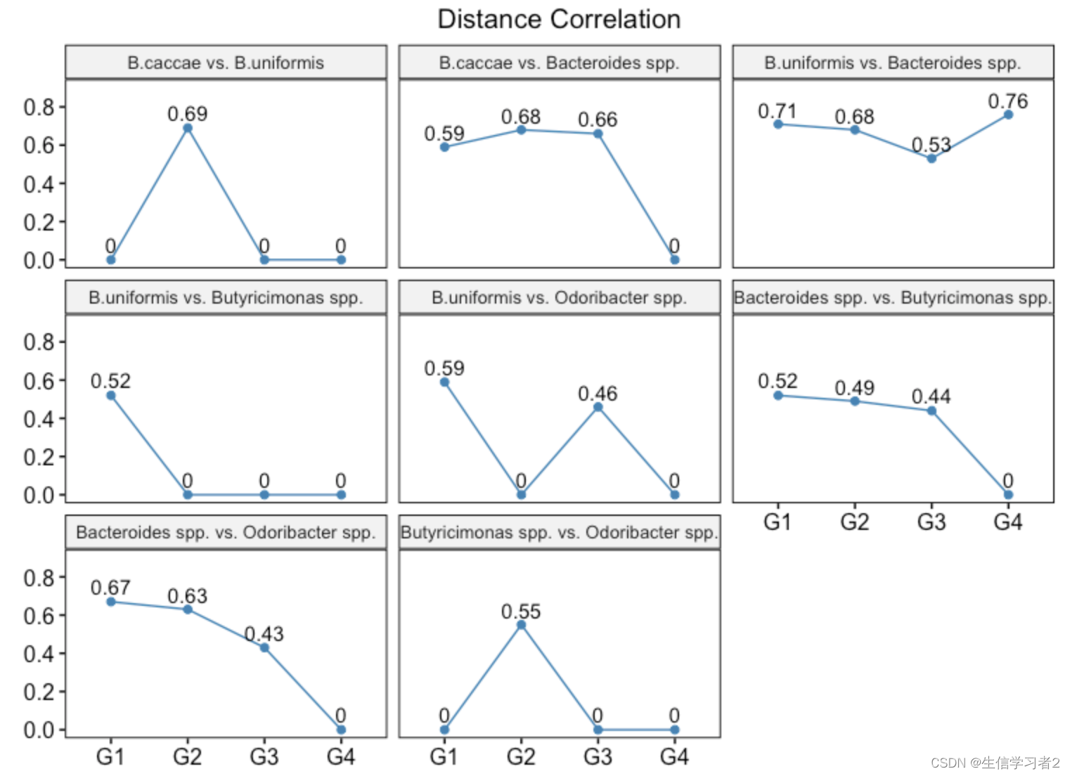
結果:同一微生物對兩兩之間的相關關系在不同分組不同,這可能表明不同狀態下,微生物之間的相關關系不一樣或意味著不同的微生物模式。
B.caccae vs. Bacteroides spp.的距離相關系數在G2組是0.68,而在G4組則是0,相比G4組,其他三個組是較為輕微的癥狀。同樣的發現也在Bacteroides spp. vs. Butyricimonas spp.和Bacteroides spp. vs. Odoribacter spp.中出現。
)


)


)