Python | 計算位渦平流項

寫在前面

最近忙著復習、考試…都沒怎么空敲代碼，還得再準備一周考試。。。等考完試再慢慢更新了，今天先來淺更一個簡單但是使用的python code

在做動力機制分析時，我們常常需要借助收支方程來診斷不同過程的貢獻，其中最常見的一項就包括水平平流項，如下所示，其中var表示某一個變量，V表示水平風場。

$-V\cdot\mathbf{\nabla}var$

以位渦的水平平流項為例，展開為

$-(u\frac{\partial pv}{\partial x}+v\frac{\partial pv}{\partial y})$

其物理解釋為：

位渦受背景氣流的調控作用。在存在背景氣流的情況下，這個位渦信號受到多少平流的貢獻

對于這種診斷量的計算，平流項，散度項，都可以通過metpy來計算。之前介紹過一次，因為metpy為大大簡便了計算

advection

但是，如果這樣還是不放心應該怎么辦呢，這里可以基于numpy的方式自己來手動計算平流項，然后比較兩種方法的差異。下面我就從兩種計算方式以及檢驗方式來計算pv的水平平流項

首先來導入基本的庫和數據，我這里用的wrf輸出的風場以及位渦pv,同時，為了減少計算量，對于數據進行區域和高度層的截取

經緯度可以直接從nc數據中獲取，我下面是之前的代碼直接拿過來用了，還是以wrf*out數據來提取的lon&lat

import numpy as np
import pandas as pd
import xarray as xr
import matplotlib.pyplot as plt
import cartopy.crs as ccrs
import glob
from matplotlib.colors import ListedColormap 
from wrf import getvar,pvo,interplevel,destagger,latlon_coords
from cartopy.mpl.ticker import LongitudeFormatter,LatitudeFormatter
from netCDF4 import Dataset
import matplotlib as mpl   
from metpy.units import units
import metpy.constants as constants
import metpy.calc as mpcalc
import cmaps
# units.define('PVU = 1e-6 m^2 s^-1 K kg^-1 = pvu')
import cartopy.feature as cfeature
f_w   = r'L:\JAS\wind.nc'
f_pv  = r'L:\JAS\pv.nc'
def  cal_dxdy(file):ncfile = Dataset(file)P = getvar(ncfile, "pressure")lats, lons = latlon_coords(P)lon = lons[0]lon[lon<=0]=lon[lon<=0]+360lat = lats[:,0]dx, dy = mpcalc.lat_lon_grid_deltas(lon.data, lat.data)return lon,lat,dx,dy
path  = r'L:\\wrf*'
filelist = glob.glob(path)
filelist.sort()
lon,lat,_,_ = cal_dxdy(filelist[-1]) 
dw = xr.open_dataset(f_w).sel(level=850,lat=slice(0,20),lon=slice(100,150))
dp = xr.open_dataset(f_pv).sel(level=850,lat=slice(0,20),lon=slice(100,150))
u = dw.u.sel(lat=slice(0,20),lon=slice(100,150))
v = dw.v.sel(lat=slice(0,20),lon=slice(100,150))
pv = dp.pv.sel(lat=slice(0,20),lon=slice(100,150))
lon = u.lon
lat = u.lat

metpy

###############################################################################
#####                  
#####                      using metpy to calculate advection
#####
###############################################################################
tadv = mpcalc.advection(pv*units('pvu'), u*units('m/s'), v*units('m/s'))
print(tadv)
###############################################################################
#####                  
#####                       plot advection
#####
###############################################################################
# start figure and set axis
fig, (ax) = plt.subplots(1, 1, figsize=(8, 6),dpi=200, subplot_kw={'projection': ccrs.PlateCarree()})
proj = ccrs.PlateCarree()
# plot isotherms
cs = ax.contour(lon, lat, pv[-1]*10**4, 8, colors='k',linewidths=0.2)
ax.coastlines('10m',linewidths=0.5,facecolor='w',edgecolor='k')
box = [100,121,0,20]
ax.set_extent(box,crs=ccrs.PlateCarree())
ax.set_xticks(np.arange(box[0],box[1], 10), crs=proj)
ax.set_yticks(np.arange(box[2], box[3], 5), crs=proj)
ax.xaxis.set_major_formatter(LongitudeFormatter())
ax.yaxis.set_major_formatter(LatitudeFormatter())
# plot tmperature advection and convert units to Kelvin per 3 hours
cf = ax.contourf(lon, lat,   tadv[10]*10**4, np.linspace(-4, 4, 21), extend='both',cmap='RdYlGn', alpha=0.75)
plt.colorbar(cf, pad=0.05, aspect=20,shrink=0.75)
ax.set_title('PV Advection Calculation')
plt.show()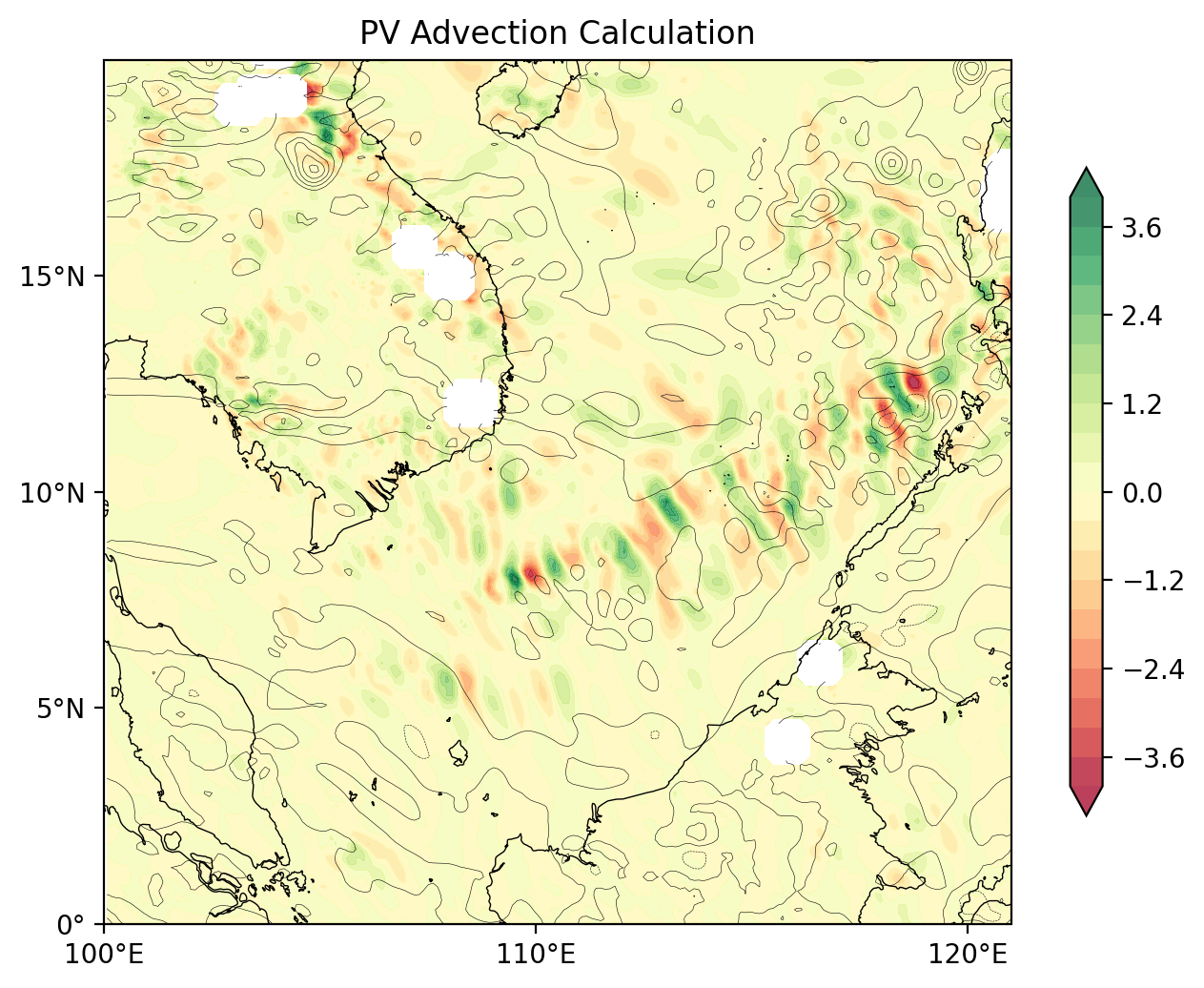

pv advection with metpy

metpy官網也提供了計算示例：

https://unidata.github.io/MetPy/latest/examples/calculations/Advection.html

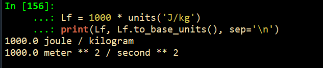
當然，這里需要提醒的是，在使用metpy計算時，最好是將變量帶上單位，這樣可以保證計算結果的量級沒有問題；或者最后將其轉換為國際基本單位:m , s ,g ...

關于metpt中單位unit的使用，可以在官網進行查閱：

https://unidata.github.io/MetPy/latest/tutorials/unit_tutorial.html

Lf = 1000 * units('J/kg')
print(Lf, Lf.to_base_units(), sep='\n')1000.0 joule / kilogram
1000.0 meter ** 2 / second ** 2

units convert

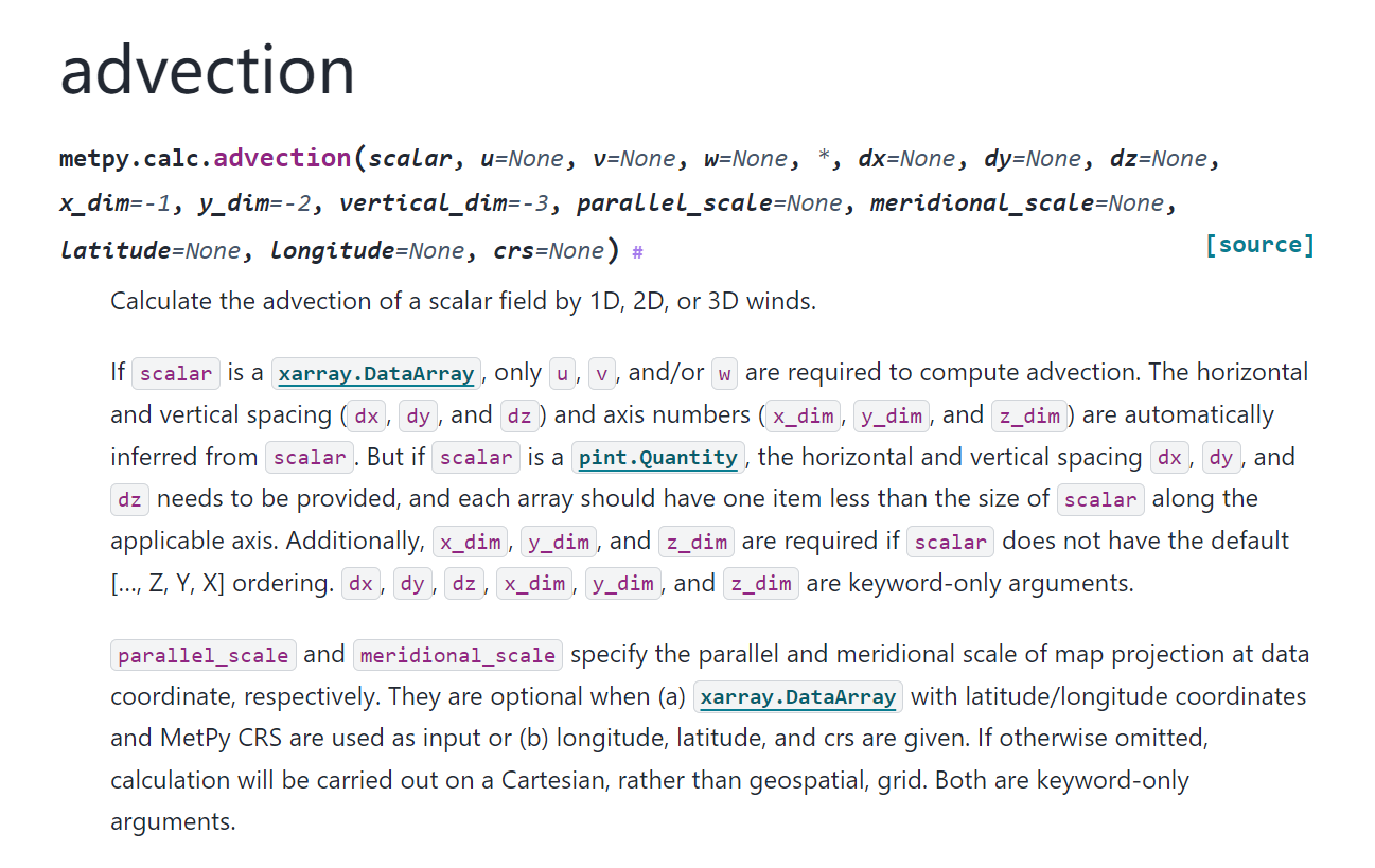
當然，還可以點擊 source code 去了解這個函數背后的計算過程：

https://github.com/Unidata/MetPy/blob/v1.6.2/src/metpy/calc/kinematics.py#L359-L468

def advection(scalar,u=None,v=None,w=None,*,dx=None,dy=None,dz=None,x_dim=-1,y_dim=-2,vertical_dim=-3,parallel_scale=None,meridional_scale=None
):r"""Calculate the advection of a scalar field by 1D, 2D, or 3D winds.If ``scalar`` is a `xarray.DataArray`, only ``u``, ``v``, and/or ``w`` are requiredto compute advection. The horizontal and vertical spacing (``dx``, ``dy``, and ``dz``)and axis numbers (``x_dim``, ``y_dim``, and ``z_dim``) are automatically inferred from``scalar``. But if ``scalar`` is a `pint.Quantity`, the horizontal and verticalspacing ``dx``, ``dy``, and ``dz`` needs to be provided, and each array should have oneitem less than the size of ``scalar`` along the applicable axis. Additionally, ``x_dim``,``y_dim``, and ``z_dim`` are required if ``scalar`` does not have the default[..., Z, Y, X] ordering. ``dx``, ``dy``, ``dz``, ``x_dim``, ``y_dim``, and ``z_dim``are keyword-only arguments.``parallel_scale`` and ``meridional_scale`` specify the parallel and meridional scale ofmap projection at data coordinate, respectively. They are optional when (a)`xarray.DataArray` with latitude/longitude coordinates and MetPy CRS are used as inputor (b) longitude, latitude, and crs are given. If otherwise omitted, calculationwill be carried out on a Cartesian, rather than geospatial, grid. Both are keyword-onlyarguments.Parameters----------scalar : `pint.Quantity` or `xarray.DataArray`The quantity (an N-dimensional array) to be advected.u : `pint.Quantity` or `xarray.DataArray` or NoneThe wind component in the x dimension. An N-dimensional array.v : `pint.Quantity` or `xarray.DataArray` or NoneThe wind component in the y dimension. An N-dimensional array.w : `pint.Quantity` or `xarray.DataArray` or NoneThe wind component in the z dimension. An N-dimensional array.Returns-------`pint.Quantity` or `xarray.DataArray`An N-dimensional array containing the advection at all grid points.Other Parameters----------------dx: `pint.Quantity` or None, optionalGrid spacing in the x dimension.dy: `pint.Quantity` or None, optionalGrid spacing in the y dimension.dz: `pint.Quantity` or None, optionalGrid spacing in the z dimension.x_dim: int or None, optionalAxis number in the x dimension. Defaults to -1 for (..., Z, Y, X) dimension ordering.y_dim: int or None, optionalAxis number in the y dimension. Defaults to -2 for (..., Z, Y, X) dimension ordering.vertical_dim: int or None, optionalAxis number in the z dimension. Defaults to -3 for (..., Z, Y, X) dimension ordering.parallel_scale : `pint.Quantity`, optionalParallel scale of map projection at data coordinate.meridional_scale : `pint.Quantity`, optionalMeridional scale of map projection at data coordinate.Notes-----This implements the advection of a scalar quantity by wind:.. math:: -\mathbf{u} \cdot \nabla = -(u \frac{\partial}{\partial x}+ v \frac{\partial}{\partial y} + w \frac{\partial}{\partial z}).. versionchanged:: 1.0Changed signature from ``(scalar, wind, deltas)``"""# Set up vectors of provided componentswind_vector = {key: valuefor key, value in {'u': u, 'v': v, 'w': w}.items()if value is not None}return_only_horizontal = {key: valuefor key, value in {'u': 'df/dx', 'v': 'df/dy'}.items()if key in wind_vector}gradient_vector = ()# Calculate horizontal components of gradient, if neededif return_only_horizontal:gradient_vector = geospatial_gradient(scalar, dx=dx, dy=dy, x_dim=x_dim, y_dim=y_dim,parallel_scale=parallel_scale,meridional_scale=meridional_scale,return_only=return_only_horizontal.values())# Calculate vertical component of gradient, if neededif 'w' in wind_vector:gradient_vector = (*gradient_vector,first_derivative(scalar, axis=vertical_dim, delta=dz))return -sum(wind * gradientfor wind, gradient in zip(wind_vector.values(), gradient_vector))

Numpy

下面，是基于numpy或者說從他的平流表達式來進行計算,下面圖方便直接將其封裝為函數了：

###############################################################################
#####                  
#####                      using numpy to calculate advection
#####
###############################################################################
def advection_with_numpy(lon,lat,pv):xlon,ylat=np.meshgrid(lon,lat)dlony,dlonx=np.gradient(xlon)dlaty,dlatx=np.gradient(ylat)pi=np.pire=6.37e6dx=re*np.cos(ylat*pi/180)*dlonx*pi/180dy=re*dlaty*pi/180pv_dx = np.gradient(pv,axis=-1)pv_dy = np.gradient(pv,axis=-2)padv_numpy = np.full((pv.shape),np.nan)for i in range(40):padv_numpy[i] = -(u[i]*pv_dx[i]/dx+v[i]*pv_dy[i]/dy)return    padv_numpy
padv = advection_with_numpy(lon, lat, pv)
###############################################################################
#####                  
#####                      check calculate advection
#####
###############################################################################
plt.figure(figsize=(10, 6),dpi=200)
plt.plot( tadv[0,0], label='adv_mean', color='blue')
plt.plot( padv[0,0], label='pvadv_mean', color='red')plt.show()

check resuly

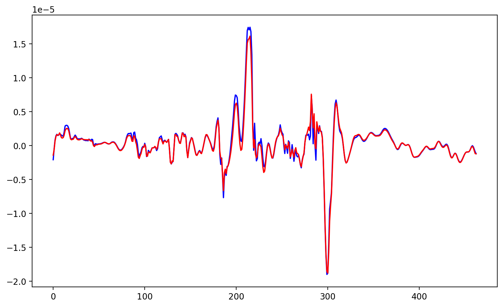
可以發現兩種方法的曲線基本一致

方法檢驗

對于兩種計算方法的計算結果進行檢驗，前面也簡單畫了一下圖，下面主要從空間分布圖以及任意選擇一個空間點的時間序列來檢驗其計算結果是否存在差異。

空間分布圖

def plot_contour(ax, data, label, lon, lat, levels, cmap='RdYlGn', transform=ccrs.PlateCarree(), extend='both'):cs = ax.contourf(lon, lat, data, levels=levels, cmap=cmap, transform=transform, extend=extend)ax.coastlines()ax.add_feature(cfeature.BORDERS)ax.set_title(label)box = [100,120,10,20]ax.set_extent(box,crs=ccrs.PlateCarree())ax.set_xticks(np.arange(box[0],box[1], 10), crs=transform)ax.set_yticks(np.arange(box[2], box[3], 5), crs=transform)ax.xaxis.set_major_formatter(LongitudeFormatter())ax.yaxis.set_major_formatter(LatitudeFormatter())plt.colorbar(cs, ax=ax, orientation='horizontal')ax.set_aspect(1)
# 創建畫布和子圖
fig, (ax1, ax2, ax3) = plt.subplots(1, 3, figsize=(16, 6),dpi=200, subplot_kw={'projection': ccrs.PlateCarree()})# 繪制三個不同的圖
plot_contour(ax1, tadv[0] * 10**4, 'Metpy', lon, lat, levels=np.linspace(-1, 1, 21))
plot_contour(ax2, padv[0] * 10**4, 'Numpy', lon, lat, levels=np.linspace(-1, 1, 21))
plot_contour(ax3, (np.array(tadv[0]) - padv[0]) * 10**4, 'difference',lon, lat, levels=11)# 顯示圖形
plt.tight_layout()
plt.show()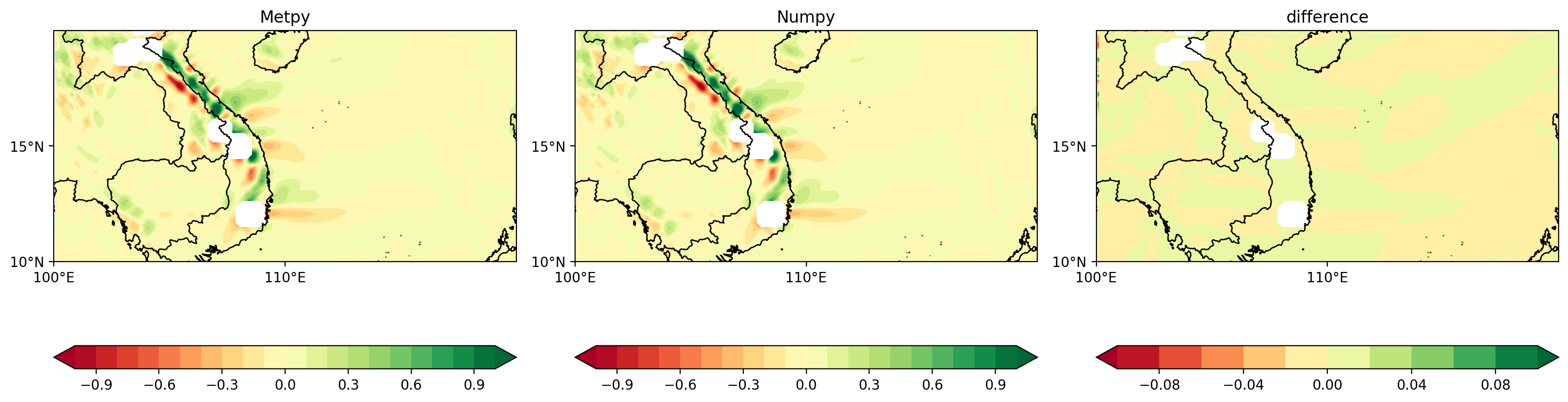

空間分布

子圖1為metpy計算結果，子圖2為numpy計算結果，子圖3為兩種計算結果的差異
為了保證結果可靠性，前兩個子圖選擇相同的量級，繪制間隔(levels)，colormap

可以發現，整體上對于第一個時刻的pv平流項空間分布圖，兩種方法的計算結果整體上是一致的，說明兩種計算方法都是可行的；兩種計算方法的差異小于0.01，在一定程度上可以忽略，不影響整體結論以及后續的分析。

任意空間點的時間序列


def extract_time_series(lon, lat, lon0, lat0, tadv, padv2):def find_nearest(array, value):array = np.asarray(array)idx = (np.abs(array - value)).argmin()return idxlon_idx = find_nearest(lon, lon0)lat_idx = find_nearest(lat, lat0)tadv_series = tadv[:, lat_idx, lon_idx] * 10**4padv2_series = padv2[:, lat_idx, lon_idx] * 10**4diff_series = (np.array(tadv[:, lat_idx, lon_idx]) - padv2[:, lat_idx, lon_idx]) * 10**4return tadv_series, padv2_series, diff_serieslon0, lat0 = 100, 15  # 根據實際需要修改# 提取該點的時間序列數據
tadv_series, padv_series, diff_series = extract_time_series(lon, lat, lon0, lat0, tadv, padv)# 創建新的畫布繪制時間序列曲線
plt.figure(figsize=(10, 6),dpi=200)
plt.plot(tadv_series, label='Metpy')
plt.plot(padv_series, label='Numpy')
plt.plot(diff_series, label='Diff')
plt.xlabel('Time')
plt.ylabel('Value')
plt.legend()
plt.title(f'Time Series at Point ({lon0}, {lat0})')
plt.grid(True)
plt.show()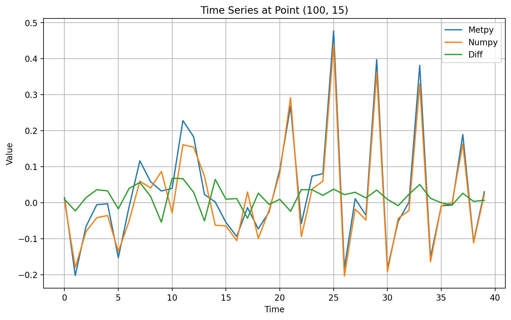

時間序列檢驗

從任意空間點的時間序列檢驗上，可以發現兩種計算方法差異基本一致，總體上Metpy的結果稍微高于numpy的計算方法，可以和地球半徑以及pi的選擇有關
從差異上來看，總體上在-0.1~0.1之間，誤差可以忽略，不會影響主要的結論

總結

這里，通過基于Metpy和Numpy的方法分別計算了位渦的平流項，并繪制了空間分布圖以及任意空間點時間序列曲線來證明兩種方法的有效性，在計算過程我們需要重點關注的是單位是否為國際基本度量單位，這里避免我們的計算的結果的量級的不確定性；
當然，這里僅僅是收支方程中的一項，我們可以在完整的計算整個收支方程的各項結果后，比較等號兩端的單位是否一致，來證明收支方程結果的有效性。

單位查閱：https://unidata.github.io/MetPy/latest/tutorials/unit_tutorial.html
advection：https://unidata.github.io/MetPy/latest/api/generated/metpy.calc.advection.html